A quadratic loss (1/2) x-transpose S x - b-transpose x has its lowest point where S x = b, exactly when S is positive definite. Derive the gradient, test flat points by their second partials, read level sets as ellipses along the eigenvectors, and measure distance in units of the data’s own ellipse.
M03.4.4L2 Intermediate25 minIn review (what this means)
The maths and code on this page are checked by automated tests on every change, but an independent reader has not signed it off yet. Spot a mistake or a confusing step? Tell us.
Derive the gradient S x - b of f(x) = (1/2) x-transpose S x - b-transpose x from its partial derivatives.
Prove that f has a unique lowest point S^(-1) b exactly when S is positive definite, by completing the square in matrix form.
Classify the flat points of a function of two variables with the matrix of its second partial derivatives.
Find the semi-axes of a level set from the eigenvalues, and compute a Mahalanobis distance.
The question
The loss of least squares and of ridge regression is, after expanding, a quadratic function of the weights: \({\tfrac12\vect{w}\T\mat{S}\vect{w} - \vect{b}\T\vect{w}}\) plus a constant. Where is its lowest point, when is there exactly one, and why does gradient descent sometimes wander towards it in a zigzag instead of heading straight there?
From the last lesson
1. Give the formulas for the 2 by 2 Cholesky factor of the matrix with rows \({(a, b)}\) and \({(b, c)}\).
2. How do you solve \({\mat{S}\vect{x} = \vect{b}}\) once you have \(\mat{L}\)?
Show answer
Forward substitution for \({\mat{L}\vect{z} = \vect{b}}\), then back substitution for \({\mat{L}\T\vect{x} = \vect{z}}\).
Intuition
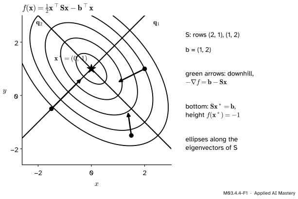
A positive definite form is a bowl with its bottom at the origin. Subtract a linear term \({\vect{b}\T\vect{x}}\) and the bowl tilts: its bottom slides to a new place and sinks below zero, but it keeps its shape. The contour lines are the same ellipses as before, only moved.
M03.4.4-F1
The quadratic loss of the worked example. The bottom is where the gradient \({\mat{S}\vect{x} - \vect{b}}\) vanishes, and the contour lines are ellipses whose axes lie along the eigenvectors of \(\mat{S}\).
Three questions follow, and this lesson answers each with something from the earlier lessons. Where is the bottom? Where the gradient is zero. Is it really a bottom? Yes, if \(\mat{S}\) is positive definite. What shape are the contour lines? Ellipses, whose axes come from the eigenvalues.
Build it up
Step 1. The gradient, one partial at a time. In two variables write \(\mat{S} = \begin{bmatrix} s_{11} & s_{12} \\ s_{12} & s_{22} \end{bmatrix}\) and \({\vect{b} = (b_1, b_2)}\), so that
(the half of the cross term \(2s_{12}xy\) is \(s_{12}xy\)). Differentiate with \(y\) held fixed, then with \(x\) held fixed (M04.10). With \(y\) fixed, \(\tfrac12 s_{11}x^2\) gives \(s_{11}x\), the term \(s_{12}xy\) gives \(s_{12}y\), the \(y^2\) term gives 0 and \({-b_1x}\) gives \({-b_1}\); the partial in \(y\) is found the same way:
These are the two rows of \({\mat{S}\vect{x} - \vect{b}}\). So \({\nabla f = \mat{S}\vect{x} - \vect{b}}\): the factor \(\tfrac12\) is there to cancel the 2 that differentiating a square produces.
Step 2. The flat point. The gradient is zero where \({\mat{S}\vect{x} = \vect{b}}\). A positive definite \(\mat{S}\) is invertible (M03.4.2), so there is exactly one such point, \({\vect{x}^* = \mat{S}^{-1}\vect{b}}\). In practice it is found by Cholesky and two triangular solves, never by forming \({\mat{S}^{-1}}\).
Step 3. The second partials are the matrix. Differentiate once more: \({\partial^2 f/\partial x^2 = s_{11}}\), \({\partial^2 f/\partial x\,\partial y = s_{12}}\) and \({\partial^2 f/\partial y^2 = s_{22}}\). For a quadratic, the matrix of second partial derivatives is \(\mat{S}\) itself, the same at every point. That is the curvature of the bowl.
Step 4. The test for any function. Near a flat point, a smooth function looks like its second-order part, a quadratic form in the step away from the point, with the matrix of second partials as its matrix (the full story, with the Hessian, is M05.5). So at a flat point: positive definite second partials mean a minimum; indefinite means a saddle. In two variables, positive definite means \({f_{xx} > 0}\) and \({f_{xx}f_{yy} - f_{xy}^2 > 0}\), the calculus test.
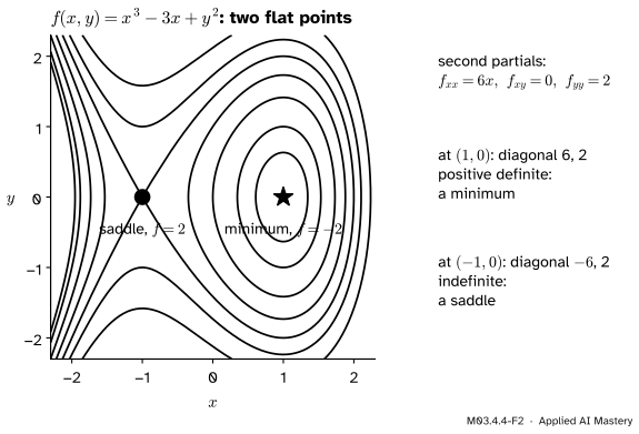
M03.4.4-F2
Two flat points of one function. The matrix of second partials is positive definite at one and indefinite at the other.
For \({f = x^3 - 3x + y^2}\) the partials are \({3x^2 - 3}\) and \({2y}\), zero at \({(1, 0)}\) and \({(-1, 0)}\). The second partials are \({f_{xx} = 6x}\), \({f_{xy} = 0}\), \({f_{yy} = 2}\). At \({(1, 0)}\) the matrix has diagonal 6 and 2: a minimum, with \({f = 1 - 3 = -2}\). At \({(-1, 0)}\) the diagonal is \({-6}\) and 2: a saddle, with \({f = -1 + 3 = 2}\).
The formal statement
NoteTheorem: the lowest point of a quadratic
Let \(\mat{S}\) be symmetric and \({f(\vect{x}) = \tfrac12\vect{x}\T\mat{S}\vect{x} - \vect{b}\T\vect{x}}\). Then \({\nabla f = \mat{S}\vect{x} - \vect{b}}\). If \(\mat{S}\) is positive definite, \(f\) has exactly one lowest point \({\vect{x}^* = \mat{S}^{-1}\vect{b}}\), with \({f(\vect{x}^*) = -\tfrac12\vect{b}\T\vect{x}^*}\), and for every \(\vect{x}\)
If \(\mat{S}\) has a negative eigenvalue, \(f\) has no lowest point. If \(\mat{S}\) is semidefinite with a zero eigenvalue, \(f\) has either no lowest point or a whole line of them. So the lowest point is unique exactly when \(\mat{S}\) is positive definite.
Proof. Expand the right-hand side and use \({\mat{S}\vect{x}^* = \vect{b}}\). The two middle terms are equal numbers, because \(\mat{S}\) is symmetric and a number equals its transpose:
At \({\vect{x} = \vect{x}^*}\) the left side is 0, so \({f(\vect{x}^*) = -\tfrac12\vect{b}\T\vect{x}^*}\), and the identity is proved. Since \(\mat{S}\) is positive definite, the right side of the theorem is positive whenever \({\vect{x} \neq \vect{x}^*}\): every other point is higher. If instead \({\mat{S}\vect{q} = \lambda\vect{q}}\) with \({\lambda < 0}\) and \({\norm{\vect{q}} = 1}\), then along \({\vect{x} = \vect{x}_0 + t\vect{q}}\) from any point \(\vect{x}_0\) the function is a parabola in \(t\) with leading term \({\tfrac12\lambda t^2}\), which falls without limit. Finally, if \({\mat{S}\vect{q} = \vect{0}}\) with \({\vect{q} \neq \vect{0}}\), expand \(f\) along the same line. The terms \({t\,\vect{q}\T\mat{S}\vect{x}_0}\) and \({\tfrac12 t^2\,\vect{q}\T\mat{S}\vect{q}}\) vanish, because \({\vect{q}\T\mat{S} = {(\mat{S}\vect{q})\T} = \vect{0}\T}\), so \({f(\vect{x}_0 + t\vect{q}) = f(\vect{x}_0) - t\,\vect{b}\T\vect{q}}\). If \({\vect{b}\T\vect{q} \neq 0}\) this falls without limit in one direction; if \({\vect{b}\T\vect{q} = 0}\) it is constant, so any lowest point \(\vect{x}_0\) comes with a whole line of others. \(\square\)
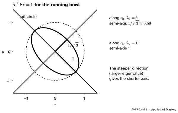
Level sets are ellipses. The level set \({f(\vect{x}) = f(\vect{x}^*) + k}\) with \({k > 0}\) is \({(\vect{x} - \vect{x}^*)\T\mat{S}(\vect{x} - \vect{x}^*) = 2k}\). In eigen-coordinates \({\vect{y} = \mat{Q}\T(\vect{x} - \vect{x}^*)}\) it reads \({\lambda_1y_1^2 + \lambda_2y_2^2 = 2k}\), an ellipse with semi-axes \({\sqrt{2k/\lambda_i}}\) along \(\vect{q}_i\). For the plain form \({\vect{x}\T\mat{S}\vect{x} = 1}\) the semi-axes are \({1/\sqrt{\lambda_i}}\): a large eigenvalue, a steep direction, a short axis.
M03.4.4-F3
The level set \({\vect{x}\T\mat{S}\vect{x} = 1}\) of the running bowl. The semi-axis along each eigenvector is one over the square root of its eigenvalue.
Distance in units of the data. For data with mean \(\vect{\mu}\) and covariance \(\mat{C}\) (positive definite), the Mahalanobis distance of a point is
Let \(\lambda_i\) be the eigenvalues of \(\mat{C}\): the variances of the data along its principal directions \(\vect{q}_i\). Then \({\mat{C}^{-1}}\) has the same eigenvectors and eigenvalues \({1/\lambda_i}\), so the set \({d = 1}\) is an ellipse with semi-axes \({\sqrt{\lambda_i}}\): one standard deviation along each principal direction of the data. Distance 2 means twice the data’s own spread, whatever the direction. The density of the multivariate Gaussian (M07.3) has \({-d^2/2}\) in its exponent, and \(d\) is a standard score for spotting outliers.
Worked example
Minimise\(f\) for the running bowl and \({\vect{b} = (1, 2)}\). The inverse of \(\mat{S}\) is \({\tfrac13}\) times the matrix with rows \({(2, -1)}\) and \({(-1, 2)}\), so
Check directly: \({f(0, 1) = \tfrac12 \cdot 2 - 2 = -1}\), and the gradient there is \({\mat{S}(0, 1) - \vect{b}} = {(1, 2) - (1, 2)} = \vect{0}\). The contour line \({f = 0}\) is the level \({k = 1}\), an ellipse round \({(0, 1)}\) with semi-axes \({\sqrt{2/3} \approx 0.82}\) along \(\vect{q}_1\) and \({\sqrt2 \approx 1.41}\) along \(\vect{q}_2\).
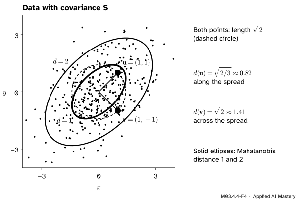
Mahalanobis distance. Take data with mean \(\vect{0}\) and covariance \({\mat{C} = \mat{S}}\), and the two points \({\vect{u} = (1, 1)}\) and \({\vect{v} = (1, -1)}\), both at ordinary distance \(\sqrt2\). With \({\mat{C}^{-1} = \tfrac13}\) times the matrix with rows \({(2, -1)}\) and \({(-1, 2)}\):
So \({d(\vect{u}) \approx 0.82}\) and \({d(\vect{v}) \approx 1.41}\). The point \(\vect{u}\) lies along the direction in which the data spread widely (variance 3), so it is unremarkable; \(\vect{v}\) lies across it (variance 1), so it is further out in the data’s own units.
M03.4.4-F4
The Mahalanobis worked example. Both black points lie on the same circle, but only \(\vect{u}\) is inside the data’s ellipse of distance 1.
Code
From scratch first: the gradient formula against finite differences, the lowest point by solving, and the level-set semi-axes.
import numpy as npS = np.array([[2.0, 1.0], [1.0, 2.0]])b = np.array([1.0, 2.0])f =lambda x: 0.5* x @ S @ x - b @ xgrad =lambda x: S @ x - bdef numeric_grad(func, x, h=1e-6): e = np.eye(len(x))return np.array([(func(x + h * e[i]) - func(x - h * e[i])) / (2* h) for i inrange(len(x))])p = np.array([2.0, -1.5])print("formula:", grad(p), " finite differences:", numeric_grad(f, p).round(6))x_star = np.linalg.solve(S, b)print("x* =", x_star, " f(x*) =", f(x_star), " -b.x*/2 =", -0.5* b @ x_star)lam, Q = np.linalg.eigh(S)print("semi-axes of x^T S x = 1:", (1/ np.sqrt(lam)).round(4), "for eigenvalues", lam)print("semi-axes of the contour f = 0:", np.sqrt(2*1.0/ lam).round(4))
formula: [ 1.5 -3. ]   finite differences: [ 1.5 -3. ]
x* = [0. 1.]   f(x*) = -1.0   -b.x*/2 = -1.0
semi-axes of x^T S x = 1: [1.     0.5774] for eigenvalues [1. 3.]
semi-axes of the contour f = 0: [1.4142 0.8165]
Now the libraries. scipy.optimize.minimize uses BFGS by default when there are no bounds or constraints; it only approximates the answer that solving gives exactly. Then the Mahalanobis distance, which SciPy’s function takes with the inverse covariance, and the second-partials test.
from scipy.optimize import minimizefrom scipy.spatial.distance import mahalanobisresult = minimize(f, x0=np.array([3.0, -2.0]), jac=grad)print("minimize:", result.x.round(6), " value:", round(result.fun, 6))C_inv = np.linalg.inv(S) # data with covariance C = Su, v = np.array([1.0, 1.0]), np.array([1.0, -1.0])for name, point in (("u", u), ("v", v)): by_hand = np.sqrt(point @ np.linalg.solve(S, point))print(name, "Mahalanobis:", round(by_hand, 4), " scipy:", round(mahalanobis(point, [0, 0], C_inv), 4)," ordinary:", round(np.linalg.norm(point), 4))def second_partials(x, y): # for f(x, y) = x^3 - 3x + y^2return np.array([[6* x, 0.0], [0.0, 2.0]])for point in ((1.0, 0.0), (-1.0, 0.0)): eig = np.linalg.eigvalsh(second_partials(*point)) kind ="minimum"if eig.min() >0else"saddle"if eig.min() <0< eig.max() else"unclear"print(point, "eigenvalues", eig, "->", kind)
In machine learning the same reasoning runs in many dimensions: the loss of least squares has the matrix \({\mat{X}\T\mat{X}}\) (up to a constant factor), positive definite when the columns of \(\mat{X}\) are independent, so its lowest point is the unique solution of the normal equations (M03.7.1).
Explore
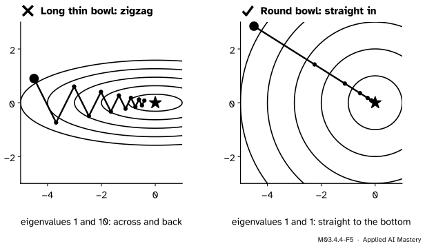
This module’s interactive, bowl or saddle, lives in lesson M03.4.2. Choose the running bowl and tap the map: the green gradient steps settle at the bottom. Then make \(c\) much larger than \(a\) to get a long thin bowl and tap again near its long axis: the steps zigzag across the valley. Choose the saddle and the steps run away along the direction of the negative eigenvalue.
Pitfalls
M03.4.4-F5
Wrong beside right. On a long thin bowl the downhill direction points mostly across the valley, so gradient descent zigzags; on a round bowl it points straight at the bottom.
“Downhill points at the minimum.”
Only on a round bowl. The gradient is at right angles to the contour line through the point, and on a long thin ellipse that direction mostly points across the valley. With eigenvalues 1 and 10, a step size large enough to make progress along the long axis overshoots across the short one, so the path zigzags. Why the speed depends on the ratio of the eigenvalues, and how rescaling the features fixes it, is the subject of M03.8.4.
“A large eigenvalue gives a long axis.”
The reverse. Along \(\vect{q}_i\) the form grows like \(\lambda_i y_i^2\), so a large \(\lambda_i\) reaches the level quickly: the semi-axis is \({1/\sqrt{\lambda_i}}\), short. For a covariance matrix it is the other way round only because the Mahalanobis distance uses \({\mat{C}^{-1}}\), whose eigenvalues are the reciprocals.
“Where the gradient is zero, the function is lowest.”
A zero gradient only makes the point flat. For \({x^3 - 3x + y^2}\) the point \({(-1, 0)}\) is flat and is a saddle. For a quadratic with an indefinite 2 by 2 \(\mat{S}\), the flat point \({\mat{S}^{-1}\vect{b}}\) exists but the function falls without limit along the negative eigenvector. Check the second partials.
Check yourself
Recall
1. What is the gradient of \({\tfrac12\vect{x}\T\mat{S}\vect{x} - \vect{b}\T\vect{x}}\) for a symmetric \(\mat{S}\)?
Show answer
\({\mat{S}\vect{x} - \vect{b}}\).
2. When does this function have exactly one lowest point, and where is it?
Show answer
When \(\mat{S}\) is positive definite. It is at \({\vect{x}^* = \mat{S}^{-1}\vect{b}}\), with value \({-\tfrac12\vect{b}\T\vect{x}^*}\).
3. How do the second partials classify a flat point of a function of two variables?
Show answer
If their matrix is positive definite (\({f_{xx} > 0}\) and \({f_{xx}f_{yy} - f_{xy}^2 > 0}\)), the point is a minimum; if it is indefinite, a saddle.
4. What are the semi-axes of the ellipse \({\vect{x}\T\mat{S}\vect{x} = 1}\)?
Show answer
\({1/\sqrt{\lambda_i}}\) along each eigenvector \(\vect{q}_i\).
5. What does a Mahalanobis distance of 1 mean?
Show answer
The point lies on the ellipse of one standard deviation of the data, whose semi-axes are the standard deviations \({\sqrt{\lambda_i}}\) along the principal directions, \(\lambda_i\) being the eigenvalues of \(\mat{C}\).
Exercises
1.★ Minimise \({\tfrac12\vect{x}\T\mat{S}\vect{x} - \vect{b}\T\vect{x}}\) for \(\mat{S}\) with rows \({(4, 2)}\) and \({(2, 3)}\) and \({\vect{b} = (6, 5)}\), and give the lowest value.
Show solution
\(\mat{S}\) is positive definite (\({4 > 0}\), \({12 - 4 = 8 > 0}\)). The lowest point solves \({\mat{S}\vect{x} = \vect{b}}\), which the last lesson solved by Cholesky: \({\vect{x}^* = (1, 1)}\). The lowest value is \({-\tfrac12(6 + 5) = -5.5}\). Check: \({\tfrac12(4 + 4 + 3) - 11} = {5.5 - 11} = -5.5\).
2.★★ Find and classify the flat points of \({f(x, y) = x^3 + y^3 - 3xy}\).
Show solution
The partials are \({3x^2 - 3y}\) and \({3y^2 - 3x}\). Zero means \({y = x^2}\) and \({x = y^2}\), so \({x = x^4}\): \({x = 0}\) or \({x = 1}\), giving \({(0, 0)}\) and \({(1, 1)}\). The second partials are \({f_{xx} = 6x}\), \({f_{xy} = -3}\), \({f_{yy} = 6y}\). At \({(0, 0)}\) the matrix has rows \({(0, -3)}\) and \({(-3, 0)}\), determinant \({-9}\): indefinite, a saddle. At \({(1, 1)}\) it has rows \({(6, -3)}\) and \({(-3, 6)}\): \({6 > 0}\) and \({36 - 9 = 27 > 0}\), positive definite, a minimum, where \({f = 1 + 1 - 3 = -1}\).
3.★★★ Show that the region \({\vect{x}\T\mat{S}\vect{x} \leq c}\) of a positive definite 2 by 2 matrix has area \({\pi c/\sqrt{\det\mat{S}}}\), and evaluate it for the running bowl with \({c = 1}\).
Show solution
The region is an ellipse with semi-axes \({\sqrt{c/\lambda_1}}\) and \({\sqrt{c/\lambda_2}}\); an ellipse with semi-axes \(p\) and \(q\) has area \({\pi pq}\). Changing to eigen-coordinates is an orthogonal change of coordinates, which keeps areas. So the area is \({\pi c/\sqrt{\lambda_1\lambda_2}} = {\pi c/\sqrt{\det\mat{S}}}\), since the determinant is the product of the eigenvalues. For the running bowl, \({\det\mat{S} = 3}\) and the area is \({\pi/\sqrt3 \approx 1.81}\).
Summary card
A positive definite matrix makes a bowl with one bottom, at \({\mat{S}\vect{x} = \vect{b}}\).
M03.4.4-F1
Bottom at \({\mat{S}\vect{x}^* = \vect{b}}\).
Gradient.\({\nabla f = \mat{S}\vect{x} - \vect{b}}\).
Minimum.\({\vect{x}^* = \mat{S}^{-1}\vect{b}}\) when \(\mat{S}\) is positive definite.
Ellipses. Semi-axes \({\sqrt{2k/\lambda_i}}\) along \(\vect{q}_i\).
Mahalanobis.\({d^2 = {\vect{u}\T\mat{C}^{-1}\vect{u}}}\) with \({\vect{u} = \vect{x} - \vect{\mu}}\).
Sources and next steps
Sources. Each was opened and checked against this lesson on 15 November 2026.
Gilbert Strang, Positive definite matrices and minima, MIT OpenCourseWare 18.06SC, lecture summary. It states that a function of several variables has a minimum where its matrix of second derivatives is positive definite, matches the 2 by 2 test with \({f_{xx}f_{yy} > f_{xy}^2}\), and says that the eigenvectors give the directions of the principal axes of the level sets and the eigenvalues their lengths (made precise above: the semi-axes of \({\vect{x}\T\mat{S}\vect{x} = 1}\) are \({1/\sqrt{\lambda_i}}\)).
SciPy reference, scipy.optimize.minimize: the default method is BFGS when there are no bounds or constraints, and the result’s x holds the solution.
SciPy reference, scipy.spatial.distance.mahalanobis: the distance \({\sqrt{(u - v)V^{-1}(u - v)\T}}\), with the argument VI the inverse of the covariance matrix.
Marc Peter Deisenroth, A. Aldo Faisal and Cheng Soon Ong, Mathematics for Machine Learning, Section 3.2.3: symmetric positive definite matrices and the forms they define.
Next. The singular value decomposition (M03.5) applies the spectral theorem to \({\mat{A}\T\mat{A}}\), a matrix this module has shown to be semidefinite. Conditioning (M03.8) explains the zigzag of the pitfall, and M05.5 extends the second-partials test with the Hessian.