Raise a matrix to any power by raising its eigenvalues instead: derive A^k = P D^k P inverse, follow a vector’s eigen-coordinates as they grow or shrink, read the long-run behaviour off the eigenvalues, and compare the cost with repeated multiplication.
M03.2.2L2 Intermediate25 minIn review (what this means)
The maths and code on this page are checked by automated tests on every change, but an independent reader has not signed it off yet. Spot a mistake or a confusing step? Tell us.
Derive A^k = P D^k P^(-1) by cancelling the inner pairs P^(-1) P, and the equivalent form A^k x = c_1 lambda_1^k v_1 + c_2 lambda_2^k v_2.
Compute a power of a 2 by 2 matrix by hand both ways and check the two answers agree.
Predict from the eigenvalues alone whether the powers of a matrix decay, grow or settle on a steady direction.
Apply a polynomial to a diagonalisable matrix through its eigenvalues, f(A) = P f(D) P^(-1).
Compare the eigen route with numpy.linalg.matrix_power in operations and in exactness.
The question
A recurrent network applies the same weight matrix at every time step, a Markov chain applies the same transition matrix at every click, and PageRank multiplies by one matrix again and again. What does a matrix do after fifty applications, or a thousand? Multiplying it out is slow and hides the answer. The eigenvalues show it at a glance.
From the last lesson
1. Why does \(\mat{A}\mat{P} = \mat{P}\mat{D}\) hold?
Show answer
Column \(j\) of \(\mat{A}\mat{P}\) is \(\mat{A}\vect{v}_j = \lambda_j\vect{v}_j\), and column \(j\) of \(\mat{P}\mat{D}\) is \(\mat{P}\) times \(\lambda_j\vect{e}_j\), which is also \(\lambda_j\vect{v}_j\).
2. What are \(\mat{P}\), \(\mat{D}\) and \(\mat{P}^{-1}\) for the running matrix \(\mat{A}\)?
Write a vector in eigen-coordinates, \(\vect{x} = {c_1\vect{v}_1 + c_2\vect{v}_2}\). One application of \(\mat{A}\) multiplies \(c_1\) by \(\lambda_1\) and \(c_2\) by \(\lambda_2\), and the two never mix. So \(k\) applications multiply them by \(\lambda_1^k\) and \(\lambda_2^k\). A matrix power, seen in the eigenbasis, is two ordinary powers of numbers.
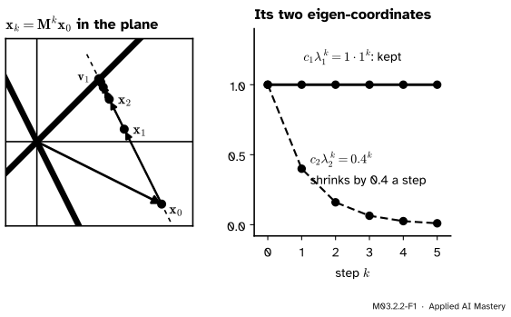
The powers of \(\mat{A}\) itself grow too fast for a picture, so take \(\mat{M} = \tfrac15\mat{A} = \begin{bmatrix} 0.8 & 0.2 \\ 0.4 & 0.6 \end{bmatrix}\). Dividing by 5 keeps the eigenvectors and divides the eigenvalues by 5: they become 1 and 0.4. (Each row of \(\mat{M}\) adds up to 1. Matrices like it are the Markov matrices of module M03.9.)
M03.2.2-F1
The powers of \(\mat{M} = \frac15\mat{A}\) applied to \(\vect{x}_0 = \vect{v}_1 + \vect{v}_2\). The part along \(\vect{v}_1\) is multiplied by 1 at every step and stays. The part along \(\vect{v}_2\) is multiplied by 0.4 and fades, so the iterates slide along a straight line onto \(\vect{v}_1\).
Every question about the long run of \(\mat{M}^k\vect{x}\) becomes a question about \(1^k\) and \(0.4^k\). The first stays 1; the second goes to 0. So the iterates settle on \(\vect{v}_1 = (1, 1)\), and the picture shows it.
Build it up
Step 1. Square the factorisation. From lesson M03.2.1, \(\mat{A} = \mat{P}\mat{D}\mat{P}^{-1}\). Then
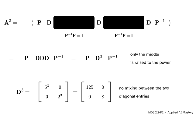
Step 3. Every power works the same way. In \(\mat{A}^k\) there are \(k\) copies of \(\mat{P}\mat{D}\mat{P}^{-1}\) and \(k - 1\) inner pairs, and each pair cancels.
M03.2.2-F2
In \(\mat{A}^3\) the two inner pairs \(\mat{P}^{-1}\mat{P}\) cancel, the three copies of \(\mat{D}\) meet in the middle, and a power of a diagonal matrix is the power of each entry.
Step 4. Powers of a diagonal matrix are free. The product of two diagonal matrices is diagonal, with entries multiplied in pairs, so
Step 5. The same fact, for one vector. Apply \(\mat{A}\) to \(\vect{x} = {c_1\vect{v}_1 + c_2\vect{v}_2}\). By linearity and \(\mat{A}\vect{v}_j = \lambda_j\vect{v}_j\), \({\mat{A}\vect{x}} = {c_1\lambda_1\vect{v}_1 + c_2\lambda_2\vect{v}_2}\). Apply it again and each term picks up one more factor. After \(k\) steps
The coefficients \(c_1, c_2\) are the eigen-coordinates of \(\vect{x}\), that is, \((c_1, c_2) = \mat{P}^{-1}\vect{x}\). So this is \(\mat{P}\mat{D}^k\mat{P}^{-1}\vect{x}\) read from the right: find the coefficients, raise the eigenvalues, rebuild.
The formal statement
NoteResult: powers of a diagonalisable matrix
If \(\mat{A} = \mat{P}\mat{D}\mat{P}^{-1}\) with \(\mat{D}\) diagonal, then for every whole number \(k \ge 1\)
\[
\mat{A}^k = \mat{P}\mat{D}^k\mat{P}^{-1},
\]
and for \(\vect{x} = c_1\vect{v}_1 + \dots + c_n\vect{v}_n\),
so it holds for \(k + 1\). For the second formula, \(\mat{A}^k\vect{v}_j = \lambda_j^k\vect{v}_j\) by the same induction (one more application multiplies by one more \(\lambda_j\)), and \(\mat{A}^k\) is linear, so it acts on each term of the sum separately. \(\blacksquare\)
The long run, read off the eigenvalues. Every term \(c_j\lambda_j^k\vect{v}_j\) behaves like the number \(\lambda_j^k\).
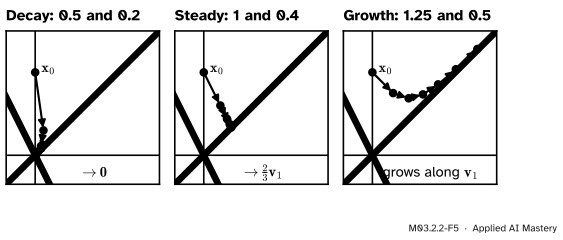
If every \(\abs{\lambda_j} < 1\), every term goes to \(\vect{0}\), so \(\mat{A}^k \to \mat{0}\): decay.
If some \(\abs{\lambda_j} > 1\) and the start has \(c_j \neq 0\), that term grows without bound: growth, along \(\vect{v}_j\).
If the largest eigenvalue is exactly 1 and all others are smaller in size, the \(\lambda = 1\) term stays and the rest fade: a steady state\(c_1\vect{v}_1\).
M03.2.2-F5
The same start under \(\frac{1}{10}\mat{A}\), \(\frac15\mat{A}\) and \(\frac14\mat{A}\), which share the eigenvectors of \(\mat{A}\) and have eigenvalues 0.5 and 0.2, 1 and 0.4, and 1.25 and 0.5. The largest eigenvalue decides the fate; the smaller one only decides how fast the iterates forget the \(\vect{v}_2\) direction.
A negative or complex eigenvalue of size 1 does not settle: \((-1)^k\) flips forever and a complex number of modulus 1 turns forever. Module M03.9 meets both.
Functions of a matrix. Since \(\mat{A}^j = \mat{P}\mat{D}^j\mat{P}^{-1}\) for each power, and \(\mat{I} = \mat{P}\mat{P}^{-1}\), any polynomial \(f(t) = {a_0 + a_1t + \dots + a_mt^m}\) gives
where \(f(\mat{D})\) is diagonal with entries \(f(\lambda_j)\). A striking case: the characteristic polynomial \(p(t) = {t^2 - 7t + 10}\) of \(\mat{A}\) has \(p(5) = p(2) = 0\), so \(p(\mat{D}) = \mat{0}\) and therefore \({\mat{A}^2 - 7\mat{A} + 10\mat{I}} = \mat{0}\) (exercise 3). Replacing the polynomial by the exponential series gives the matrix exponential \(e^{\mat{A}}\), which solves systems of differential equations; module M12.1 takes it up.
Worked example
Compute \(\mat{A}^5\) for \(\mat{A} = \begin{bmatrix} 4 & 1 \\ 2 & 3 \end{bmatrix}\), once with the whole matrix and once through one vector.
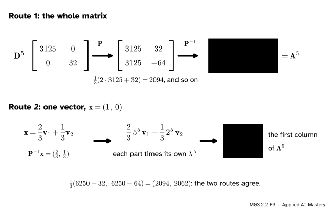
Route 1, the matrix.\(\mat{D}^5\) has entries \(5^5 = 3125\) and \(2^5 = 32\). Multiplying by \(\mat{P}\) on the left scales its columns:
Two checks from lesson M03.1.3: the trace is \({2094 + 1063} = 3157 = {3125 + 32}\), the sum of the eigenvalues of \(\mat{A}^5\), and the determinant is \({2094 \cdot 1063} - {1031 \cdot 2062} = 100000 = 10^5\).
Route 2, one vector. Take \(\vect{x} = (1, 0)\). Its eigen-coordinates are \({\mat{P}^{-1}(1, 0)} = {(\tfrac23, \tfrac13)}\), so \(\vect{x} = {\tfrac23\vect{v}_1 + \tfrac13\vect{v}_2}\).
M03.2.2-F3
The same power two ways. The whole matrix needs \(\mat{D}^5\) and two products. One vector needs only its two eigen-coordinates, each multiplied by its own eigenvalue to the fifth.
Each coordinate is multiplied by its own eigenvalue five times:
How much work is each route? The slow route uses \(k - 1\) matrix products. NumPy’s matrix_power uses repeated squaring: write \(k\) in binary, square the matrix once per binary digit, and multiply in the squares whose digit is 1. The eigen route, once \(\mat{P}\) and \(\mat{P}^{-1}\) are known, always needs two matrix products, whatever \(k\) is.
def squaring_count(k):"""Matrix products used by repeated squaring for the power k: (squarings, extra products).""" bits =bin(k)[2:]returnlen(bits) -1, bits.count("1") -1for k in (5, 20, 1000): squares, extra = squaring_count(k)print(f"k = {k:4d}: slow {k -1:3d} products, squaring {squares + extra:2d}, eigen route 2")
k =    5: slow   4 products, squaring  3, eigen route 2
k =   20: slow  19 products, squaring  5, eigen route 2
k = 1000: slow 999 products, squaring 14, eigen route 2
For \(k = 1000\): 999 products, 14 products, or 2. Now the library. With an integer array matrix_power is exact, but NumPy’s 64-bit integers hold numbers only up to about \({9.2 \times 10^{18}}\), and the entries of \(\mat{A}^{28}\) are bigger. NumPy does not warn: the answer wraps around and is simply wrong.
import numpy as npA_np = np.array([[4, 1], [2, 3]])print("A^5:\n", np.linalg.matrix_power(A_np, 5))def exact_power(k):"""Entries of A^k from the eigen formula, in Python's unlimited integers."""return [[(2*5** k +2** k) //3, (5** k -2** k) //3], [(2*5** k -2*2** k) //3, (5** k +2*2** k) //3]]for k in (27, 28):print(k, "int64 correct?", np.linalg.matrix_power(A_np, k).tolist() == exact_power(k))P_f = np.array([[1.0, 1.0], [1.0, -2.0]])eigen_30 = P_f @ np.diag([5.0**30, 2.0**30]) @ np.linalg.inv(P_f)print("float eigen route, A^30 entry (1, 2):", f"{eigen_30[0, 1]:.0f}")print("exact: ", exact_power(30)[0][1])
The float eigen route is fast but approximate: beyond \(2^{53}\) a float cannot even hold every whole number, so the last digits of \(\mat{A}^{30}\) are lost. Python’s own integers never overflow, which is why the exact formula above uses them.
Explore
M03.2-X1
Power stepper
Choose a matrix, drag the start (or use its sliders) and press step. The bars show the two eigen-coordinates \(c_1\lambda_1^k\) and \(c_2\lambda_2^k\). Switch on normalising to run the power method of lesson M03.2.4.
Things to try:
With the running matrix \(\mat{A}\), step five times from \((1, 0)\) and compare the bars with route 2 of the worked example: \(\tfrac23 \cdot 5^5\) and \(\tfrac13 \cdot 2^5\).
Choose \(\tfrac15\mat{A}\) and step until the second bar has all but vanished. The vector stops moving: a steady state.
Choose the swap matrix, whose eigenvalues are 1 and \(-1\). The second bar flips sign at every step and never shrinks.
Pitfalls
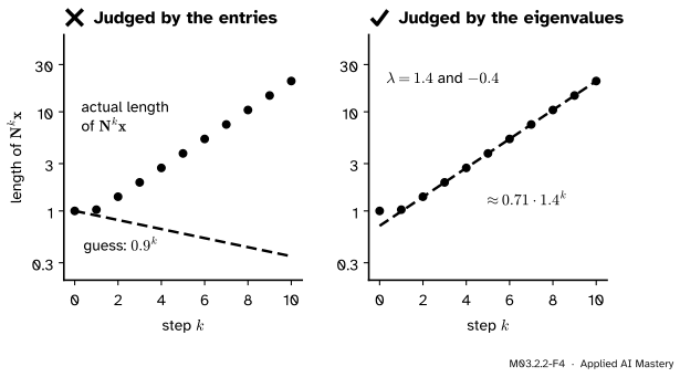
M03.2.2-F4
Wrong beside right. Every entry of \(\mat{N}\) is below 1, yet its powers grow, because its eigenvalues are 1.4 and \(-0.4\). On a log scale the lengths lie on the line \(0.71 \cdot 1.4^k\).
“All the entries are smaller than 1, so the powers shrink.”
Size is decided by the eigenvalues, not by the entries. The matrix \(\mat{N} = \begin{bmatrix} 0.5 & 0.9 \\ 0.9 & 0.5 \end{bmatrix}\) sends \((1, 1)\) to \({(1.4, 1.4)}\), so \(\lambda = 1.4\) and its powers grow like \(1.4^k\). The same mistake in the other direction is just as easy: large entries can come with small eigenvalues. This is why recurrent networks are analysed through the eigenvalues of their weight matrices.
“\(\mat{A}^k = \mat{P}^k\mat{D}^k\mat{P}^{-k}\).”
Only the middle factor is raised to the power. The outer \(\mat{P}\) and \(\mat{P}^{-1}\) appear once each, because all the inner ones cancelled. Raising \(\mat{P}\) to a power would change the basis \(k\) times over, which has nothing to do with \(\mat{A}\).
“The eigen route is exact, so I can use it for big integer powers.”
In floating point it is not: by \(\mat{A}^{30}\) the entries are far beyond \(2^{53}\) and the last digits are lost. And matrix_power on an int64 array is exact only until the entries pass about \({9.2 \times 10^{18}}\), which for \(\mat{A}\) happens at \(k = 28\), without a warning. For exact large powers use Python integers or dtype=object.
Check yourself
Recall
1. Why does \(\mat{A}^k\) equal \(\mat{P}\mat{D}^k\mat{P}^{-1}\)?
Show answer
In the product of \(k\) copies of \(\mat{P}\mat{D}\mat{P}^{-1}\), every inner pair \(\mat{P}^{-1}\mat{P}\) is the identity and drops out, leaving \(\mat{P}\mat{D}^k\mat{P}^{-1}\).
2. If \(\vect{x} = c_1\vect{v}_1 + c_2\vect{v}_2\) in eigenvectors, what is \(\mat{A}^k\vect{x}\)?
Show answer
\(c_1\lambda_1^k\vect{v}_1 + c_2\lambda_2^k\vect{v}_2\): each eigen-coordinate is multiplied by its own eigenvalue \(k\) times.
3. What do the eigenvalues say about the long run of \(\mat{A}^k\vect{x}\)?
Show answer
All of size below 1: decay to zero. One above 1 (with a non-zero coefficient): growth along its eigenvector. Largest exactly 1 and the others smaller: a steady state along the eigenvector of 1.
4. What are the first column of \(\mat{A}^5\) and its trace for the running \(\mat{A}\)?
Show answer
The first column is \((2094, 2062)\), and the trace is \(3157 = 5^5 + 2^5\).
5. How is a polynomial \(f\) applied to a diagonalisable matrix?
Show answer
\(f(\mat{A}) = \mat{P}f(\mat{D})\mat{P}^{-1}\), where \(f(\mat{D})\) is diagonal with entries \(f(\lambda_j)\).
Exercises
1.★ Compute \(\mat{A}^3\) through the eigenbasis and check it by multiplying \(\mat{A}^2 = \begin{bmatrix} 18 & 7 \\ 14 & 11 \end{bmatrix}\) by \(\mat{A}\).
Show solution
\(\mat{D}^3\) has entries 125 and 8, so \(\mat{P}\mat{D}^3 = \begin{bmatrix} 125 & 8 \\ 125 & -16 \end{bmatrix}\). Then
Check: \(\mat{A}^2\mat{A}\) has first row \({(18 \cdot 4 + 7 \cdot 2,\; 18 + 21)} = (86, 39)\) and second row \({(14 \cdot 4 + 11 \cdot 2,\; 14 + 33)} = (78, 47)\).
2.★★ For \(\mat{M} = \tfrac15\mat{A}\), find the limit of \(\mat{M}^k\) as \(k\) grows, and the limit of \(\mat{M}^k\vect{x}_0\) for \(\vect{x}_0 = (0, 2)\).
Show solution
\(\mat{M}\) has the eigenvectors of \(\mat{A}\) and eigenvalues 1 and 0.4, so \(\mat{M}^k = \mat{P}\begin{bmatrix} 1 & 0 \\ 0 & 0.4^k \end{bmatrix}\mat{P}^{-1}\). As \(0.4^k \to 0\),
So \(\mat{M}^k(0, 2) \to {\tfrac13(0 + 2,\; 0 + 2)} = {(\tfrac23, \tfrac23)} = \tfrac23\vect{v}_1\), the end point of the middle panel of the figure on long runs. Both rows of the limit are \({(\tfrac23, \tfrac13)}\): every start forgets everything except its \(\vect{v}_1\) coordinate.
3.★★★ Use \(f(\mat{A}) = \mat{P}f(\mat{D})\mat{P}^{-1}\) with \(p(t) = t^2 - 7t + 10\) to show \({\mat{A}^2 - 7\mat{A} + 10\mat{I}} = \mat{0}\). Deduce a formula for \(\mat{A}^{-1}\) that needs no determinant, and check it.
Show solution
\(p(5) = 25 - 35 + 10 = 0\) and \(p(2) = 4 - 14 + 10 = 0\), so \(p(\mat{D}) = \mat{0}\) and \(p(\mat{A}) = \mat{P}\,\mat{0}\,\mat{P}^{-1} = \mat{0}\). Rearranging, \({\mat{A}(7\mat{I} - \mat{A})} = 10\mat{I}\), so
Sources. Each was opened and checked against this lesson on 15 November 2026.
Gilbert Strang, Diagonalization and powers of A, MIT OpenCourseWare 18.06SC, lecture 22 and its lecture summary. The summary derives \(A^2 = S\Lambda^2S^{-1}\) by cancelling \(S^{-1}S\) and states \(A^k = S\Lambda^kS^{-1}\), the theorem that \(A^k \to 0\) exactly when every \(\abs{\lambda_i} < 1\) (for \(A\) with \(n\) independent eigenvectors), and the solution \(u_k = c_1\lambda_1^kx_1 + \dots + c_n\lambda_n^kx_n\) of \(u_{k+1} = Au_k\).
NumPy reference, numpy.linalg.matrix_power. For positive integers the power is computed by repeated matrix squarings and matrix multiplications, and the result has the same type as the input for a non-negative exponent.