Write a graph as its adjacency matrix and its powers count walks; write it as its Laplacian and the quadratic form adds up squared differences across edges. The zero eigenvalues count the pieces, and the second eigenvector cuts a graph into two clusters.
M03.9.3L2 Intermediate25 minIn review (what this means)
The maths and code on this page are checked by automated tests on every change, but an independent reader has not signed it off yet. Spot a mistake or a confusing step? Tell us.
Write the adjacency matrix of a directed and of an undirected graph, and read degrees off its rows.
Prove by induction that entry (i, j) of the k-th power of the adjacency matrix counts the walks of length k from i to j.
Derive x-transpose L x = sum over edges of (x_i - x_j)^2 for the Laplacian L = D - A, and conclude that it is positive semidefinite.
Count the connected pieces of a graph from the zero eigenvalues of its Laplacian, and split a graph by the signs of its Fiedler vector.
The question
Friendships, molecules, citations and road maps are all graphs: dots joined by lines. Machine learning works on them every day, clustering the members of a network into communities and passing messages along bonds in graph neural networks. How can a matrix count the routes through a graph, and how can one eigenvector find where a network naturally splits in two?
From the last lesson
1. What does the Perron-Frobenius theorem promise for a positive Markov matrix?
Show answer
A simple eigenvalue 1 with every other eigenvalue of modulus below 1, exactly one stationary distribution with positive entries, and convergence to it from every start.
2. What goes wrong for a Markov chain in two separate pieces?
Show answer
The eigenvalue 1 is repeated, there is a whole family of steady states, and the start decides which one is reached.
Intuition
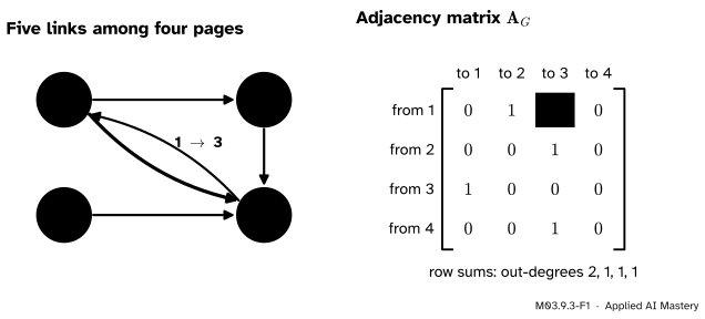
A graph is a set of nodes joined by edges. In a directed graph each edge is an arrow from one node to another, as with links between web pages. Number the nodes and write a 1 in row \(i\), column \(j\) whenever there is an arrow from \(i\) to \(j\). That table is the adjacency matrix\(\mat{A}_G\).
M03.9.3-F1
The running web of this module as a directed graph. Each arrow is one entry equal to 1: the green arrow from page 1 to page 3 is the 1 in row 1, column 3.
Nothing is lost in the translation: the picture can be redrawn from the matrix. What is gained is that matrix operations now mean something about the graph.
Build it up
Step 1. Rows and columns are out and in. Row \(i\) of \(\mat{A}_G\) lists the arrows leaving \(i\), so its sum is the out-degree of \(i\). Column \(j\) lists the arrows arriving at \(j\), so its sum is the in-degree. In the web, page 3 has in-degree 3 and page 4 has in-degree 0.
Step 2. Undirected graphs give symmetric matrices. In an undirected graph an edge joins \(i\) and \(j\) both ways, so \(a_{ij} = a_{ji}\) and \(\mat{A}_G\T = \mat{A}_G\). The number of edges at node \(i\) is its degree\(d_i\), the sum of row \(i\).
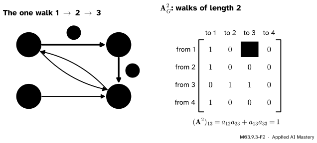
Step 3. Two steps are a product. Entry \((i, j)\) of \(\mat{A}_G^2\) is \({\sum_k a_{ik}a_{kj}}\). A term \(a_{ik}a_{kj}\) is 1 exactly when there is an arrow \(i \to k\) and an arrow \(k \to j\), and 0 otherwise. So the sum counts the two-step routes from \(i\) to \(j\).
M03.9.3-F2
Row 1 of \(\mat{A}_G\) times column 3 of \(\mat{A}_G\) adds one term for each middle page \(k\). Only \(k = 2\) gives a route, so \((\mat{A}_G^2)_{13} = 1\).
Step 4. Divide by the degrees and you have a Markov chain. Divide each row of \(\mat{A}_G\) by its out-degree. Every row now adds to 1: a walker who follows a random arrow out of each page. That Markov matrix is the start of PageRank in the next lesson.
The formal statement
NoteResult: powers count walks
A walk of length \(k\) is a sequence of \(k\) edges, each starting where the last one ended; nodes may repeat. For every \(k \ge 1\), \((\mat{A}_G^k)_{ij}\) is the number of walks of length \(k\) from \(i\) to \(j\).
Proof, by induction on \(k\). For \(k = 1\) a walk of length 1 is a single edge, and \(a_{ij}\) is 1 exactly when that edge exists. Suppose the claim holds for \(k\). Every walk of length \(k + 1\) from \(i\) to \(j\) is a walk of length \(k\) from \(i\) to some node \(m\), followed by one edge from \(m\) to \(j\). Group the walks by \(m\): for each \(m\) there are \((\mat{A}_G^k)_{im}\) choices for the first part and \(a_{mj}\) for the last edge. So the number of walks is
Node \(i\) appears in \(d_i\) edges, so \({\sum_i d_i x_i^2}\) gives each edge \(\{i, j\}\) the two terms \({x_i^2 + x_j^2}\). The adjacency part is \({\sum_{i,j} a_{ij}x_ix_j}\), and each edge appears twice in it, as \((i, j)\) and as \((j, i)\), giving \({2x_ix_j}\). Subtract, edge by edge:
Semidefinite. A sum of squares is never negative, so \(\mat{L}_G\) is positive semidefinite (M03.4.2) and, being symmetric, has real eigenvalues \({0 \le \lambda_1 \le \dots \le \lambda_n}\).
Zero comes first. For \(\vect{x} = \vect{1}\) every difference is 0, so \(\mat{L}_G\vect{1} = \vect{0}\): each row of \(\mat{L}_G\) adds to 0.
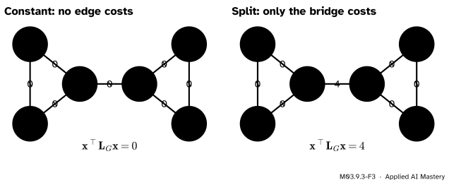
Smooth vectors are cheap. The form is small when neighbours carry similar numbers. A vector that changes sign across only a few edges costs little.
M03.9.3-F3
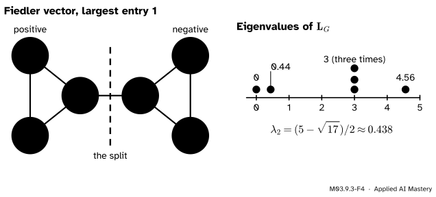
The Laplacian form adds a squared difference for every edge. A constant vector costs nothing. Putting \(+1\) on one triangle and \(-1\) on the other costs only the bridge between them.
NoteResult: zero eigenvalues count the pieces
The number of zero eigenvalues of \(\mat{L}_G\) equals the number of connected pieces of the graph, and the eigenvectors for 0 are the vectors that are constant on each piece.
Proof. If \(\mat{L}_G\vect{x} = \vect{0}\) then \({\vect{x}\T\mat{L}_G\vect{x} = 0}\), so every edge has \(x_i = x_j\), and \(\vect{x}\) is constant along every edge and hence on each piece. Conversely, a vector constant on each piece makes every term zero, so \(\vect{x}\T\mat{L}_G\vect{x} = 0\). For a semidefinite matrix that forces \(\mat{L}_G\vect{x} = \vect{0}\): write \(\mat{L}_G = {\mat{Q}\Lambda\mat{Q}\T}\) (M03.3.2), so \({\vect{x}\T\mat{L}_G\vect{x} = \sum_i \lambda_i(\vect{q}_i \cdot \vect{x})^2}\), and every term with \(\lambda_i > 0\) must vanish. Then every term of \({\mat{L}_G\vect{x} = \sum_i \lambda_i(\vect{q}_i \cdot \vect{x})\,\vect{q}_i}\) is zero too. The indicator vectors of the pieces (1 on one piece, 0 elsewhere) are independent and span these vectors, so the null space has one dimension per piece. \(\blacksquare\)
M03.9.3-F6
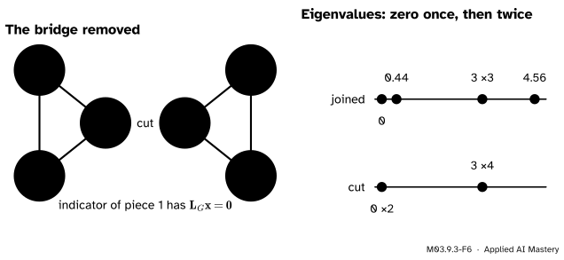
Remove the bridge and the graph falls into two pieces. The Laplacian then has the eigenvalue 0 twice, with the indicators of the two triangles as eigenvectors. The bridge lifts one of the zeros to 0.44.
Worked example
Find every eigenvalue of the Laplacian of two triangles joined by one edge, and the eigenvector that splits them.
Number the nodes as in the figures: triangle \(\{1, 2, 3\}\), triangle \(\{4, 5, 6\}\), bridge \(\{3, 4\}\). The degrees are \((2, 2, 3, 3, 2, 2)\), so the rows of \(\mat{L}_G\) are
The graph looks the same after swapping 1 with 2, or 5 with 6, or the two triangles. Use that.
Vectors that are odd within a triangle. For \((1, -1, 0, 0, 0, 0)\), row 1 gives \({2 + 1} = 3\), row 2 gives \({-1 - 2} = -3\) and row 3 gives \({-1 + 1} = 0\): the eigenvalue is 3. The same holds for \((0, 0, 0, 0, 1, -1)\).
Vectors that are the same on both triangles, \((a, a, b, b, a, a)\). Row 1 gives \({2a - a - b} = {a - b}\) and row 3 gives \({3b - 2a - b} = {2b - 2a}\). For an eigenvalue \(\lambda\), the first says \({b = (1 - \lambda)a}\); put that in the second, \({2(b - a)} = \lambda b\):
So \(\lambda = 0\) (the constant vector) or \(\lambda = 3\).
Vectors that change sign between the triangles, \((a, a, b, -b, -a, -a)\). Row 1 again gives \({a - b} = \lambda a\), so \({b = (1 - \lambda)a}\). Row 3 now gives \({3b - 2a + b} = {4b - 2a}\), so \({4b - 2a} = \lambda b\). Put in \(b\) and divide by \(a\):
So \({\lambda = (5 \pm \sqrt{17})/2}\), about \(0.438\) and \(4.562\). That is six eigenvalues in all: \(0\), \(0.438\), \(3\), \(3\), \(3\), \(4.562\). They add to 14, the trace of \(\mat{L}_G\), as they must.
The second-smallest, \(\lambda_2 \approx 0.438\), is the algebraic connectivity, and its eigenvector is the Fiedler vector. With \(a = 1\), \({b = 1 - 0.438} = 0.562\):
The Fiedler vector of two joined triangles. Its signs put nodes 1, 2, 3 on one side and 4, 5, 6 on the other, and the bridge nodes, nearest the cut, carry the values closest to zero.
Its signs split the graph exactly into the two triangles, and the only edge it cuts is the bridge. That is spectral clustering in miniature (ML03): small eigenvectors of the Laplacian vary slowly along edges, so their signs group nodes that are densely connected.
Code
From scratch: matrices from an edge list, then each claim of the lesson.
import numpy as npedges = [(1, 2), (1, 3), (2, 3), (3, 4), (4, 5), (4, 6), (5, 6)] # two triangles and a bridgen =6A = np.zeros((n, n))for i, j in edges: A[i -1, j -1] = A[j -1, i -1] =1# undirected: both waysD = np.diag(A.sum(axis=1))L = D - A# walks: every node lies on one triangle, which it can go round in two directionsA3 = np.linalg.matrix_power(A, 3)print("closed walks of length 3:", np.diag(A3), " triangles:", np.trace(A3) /6)# the quadratic form, checked against the sum over edges for a random xrng = np.random.default_rng(0)x = rng.normal(size=n)print("x'Lx =", x @ L @ x, " edge sum =", sum((x[i -1] - x[j -1]) **2for i, j in edges))
closed walks of length 3: [2. 2. 2. 2. 2. 2.]   triangles: 2.0
x'Lx = 2.496275387580259   edge sum = 2.496275387580259
Now the eigenvalues with numpy.linalg.eigh, which is made for symmetric matrices: it returns them in ascending order, with orthonormal eigenvectors as columns.
w, V = np.linalg.eigh(L)print("eigenvalues:", np.round(w, 3))fiedler = V[:, 1]print("Fiedler vector:", np.round(fiedler, 3))print("groups:", np.where(fiedler >0)[0] +1, np.where(fiedler <0)[0] +1)cut = [e for e in edges if e != (3, 4)] # remove the bridgeA_cut = np.zeros((n, n))for i, j in cut: A_cut[i -1, j -1] = A_cut[j -1, i -1] =1w_cut = np.linalg.eigvalsh(np.diag(A_cut.sum(axis=1)) - A_cut)print("without the bridge:", np.round(w_cut, 3), " zero eigenvalues:", np.sum(np.abs(w_cut) <1e-9))
The groups print in whichever order the sign of the Fiedler vector comes out: eigh may return \(-\vect{f}\) as well as \(\vect{f}\), on any machine. The ratio \(b/a\) is \({(\sqrt{17} - 3)/2} \approx 0.562\), the value found by hand.
Explore
The random surfer in lesson M03.9.4 draws the running web as a directed graph. Each link you switch off deletes a 1 from \(\mat{A}_G\), and the random walk built from it changes with it.
Pitfalls
M03.9.3-F5
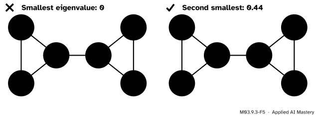
Wrong beside right. The eigenvector of the smallest eigenvalue is constant, \(1/\sqrt6 \approx 0.41\) at every node, and cannot split anything. The second one, the Fiedler vector (here scaled to length 1), does.
“The eigenvector of the smallest eigenvalue finds the clusters.”
The smallest eigenvalue of a Laplacian is always 0, with the constant vector, for every graph. Spectral clustering starts from the second-smallest. With several pieces there are several zeros, and then the eigenvectors for 0 already mark the pieces.
“\(\mat{A}_G^k\) counts paths.”
It counts walks, which may revisit nodes and edges. In the two triangles \((\mat{A}_G^2)_{33} = 3\): three walks from node 3 out along an edge and straight back. None of them is a path to anywhere.
“The Laplacian facts hold for any graph.”
They were derived for undirected graphs, where \(\mat{A}_G\) is symmetric and each edge was counted twice in \({\sum_{i,j} a_{ij}x_ix_j}\). For the directed web, \(\mat{D} - \mat{A}_G\) is not symmetric, its form is not a sum of squares and its eigenvalues can be complex. Directed graphs get their matrix in the next lesson: the random walk.
Frontier note: the Laplacian inside a graph neural network
A graph convolutional network (Kipf and Welling, 2017) updates the features \(\mat{H}\) of all nodes at once by
where \(\tilde{\mat{A}} = \mat{A}_G + \mat{I}\) adds a self-loop to each node and \(\tilde{\mat{D}}\) holds its degrees. Each layer averages a node with its neighbours, a smoothing step that the paper derives from a first-order approximation of filters on the eigenvalues of the normalised Laplacian \(\mat{I} - {\mat{D}_G^{-1/2}\mat{A}_G\mat{D}_G^{-1/2}}\), a scaled cousin of \(\mat{L}_G\). Course DL09 builds these networks.
Check yourself
Recall
1. What is entry \((i, j)\) of the adjacency matrix of a directed graph?
Show answer
1 if there is an edge from \(i\) to \(j\), and 0 otherwise. Row sums are out-degrees, column sums in-degrees.
2. What does \((\mat{A}_G^k)_{ij}\) count?
Show answer
The walks of length \(k\) from node \(i\) to node \(j\).
3. What is \(\vect{x}\T\mat{L}_G\vect{x}\) for the Laplacian of an undirected graph?
Show answer
The sum over edges \(\{i, j\}\) of \((x_i - x_j)^2\), so it is never negative.
4. What do the zero eigenvalues of a Laplacian tell you?
Show answer
Their number is the number of connected pieces, and their eigenvectors are the vectors that are constant on each piece.
5. What is the Fiedler vector, and how does it split a graph?
Show answer
The eigenvector of the second-smallest Laplacian eigenvalue. Nodes with positive entries form one group and nodes with negative entries the other.
Exercises
1.★ For the running web, compute row 1 of \(\mat{A}_G^3\) and list the walks it counts.
Show solution
Row 1 of \(\mat{A}_G^2\) is \((1, 0, 1, 0)\): one walk to page 1 (\(1 \to 3 \to 1\)) and one to page 3 (\(1 \to 2 \to 3\)). Multiply by \(\mat{A}_G\): row 1 of \(\mat{A}_G^3\) is row 1 of \(\mat{A}_G\) plus row 3 of \(\mat{A}_G\), that is \({(0, 1, 1, 0) + (1, 0, 0, 0)} = (1, 1, 1, 0)\). The walks are \(1 \to 2 \to 3 \to 1\), \(1 \to 3 \to 1 \to 2\) and \(1 \to 3 \to 1 \to 3\).
2.★★ Find the Laplacian of the path \(1 - 2 - 3\), its eigenvalues and its Fiedler vector.
Show solution
The degrees are 1, 2, 1, so the rows of \(\mat{L}_G\) are \((1, -1, 0)\), \((-1, 2, -1)\) and \((0, -1, 1)\). The constant vector gives 0. For \((1, 0, -1)\): row 1 gives 1, row 2 gives 0 and row 3 gives \(-1\), so the eigenvalue is 1. For \((1, -2, 1)\): row 1 gives \({1 + 2} = 3\), row 2 gives \({-1 - 4 - 1} = -6\) and row 3 gives 3, so the eigenvalue is 3. The eigenvalues \(0, 1, 3\) add to 4, the trace. The Fiedler vector is \((1, 0, -1)\): it puts the two ends on opposite sides, with the middle node on the cut.
3.★★★ Show that for an undirected graph with no self-loops, \({\operatorname{tr}(\mat{A}_G^3)}\) is six times the number of triangles. Check it on the two joined triangles.
Show solution
By the walk theorem, \((\mat{A}_G^3)_{ii}\) counts the closed walks of length 3 from \(i\). With no self-loops, a closed walk \(i \to j \to k \to i\) needs \(j \ne i\), \(k \ne j\) and \(k \ne i\), so \(i, j, k\) are three different nodes joined in a triangle. Conversely each triangle \(\{i, j, k\}\) gives six closed walks of length 3: three starting nodes times two directions. Summing over \(i\), \({\operatorname{tr}(\mat{A}_G^3)} = 6 \times (\text{number of triangles})\). For the two triangles every diagonal entry of \(\mat{A}_G^3\) is 2, the trace is 12, and \(12/6 = 2\) triangles.
Summary card
A graph is a matrix: powers count walks, and the Laplacian’s small eigenvectors find the pieces.
M03.9.3-F1
An arrow is a 1 in the matrix.
Adjacency.\(a_{ij} = 1\) for an edge \(i \to j\); undirected means symmetric.
Walks.\((\mat{A}_G^k)_{ij}\) = number of walks of length \(k\) from \(i\) to \(j\).
Pieces. Number of zero eigenvalues = number of connected pieces.
Clusters. The signs of the Fiedler vector split the graph.
Sources and next steps
Sources. Each was opened and checked against this lesson on 15 November 2026.
Ulrike von Luxburg, A tutorial on spectral clustering, Statistics and Computing 17 (2007). Section 3.1, Proposition 1: for \(L = D - W\), \(f\T Lf = \tfrac12\sum_{i,j} w_{ij}(f_i - f_j)^2\), \(L\) is symmetric and positive semidefinite, and its smallest eigenvalue is 0 with the constant eigenvector. Proposition 2: the multiplicity of the eigenvalue 0 equals the number of connected components, with their indicator vectors spanning the eigenspace. (Her sum runs over ordered pairs, hence the factor one half.)
Wikipedia, Algebraic connectivity: the second-smallest Laplacian eigenvalue, positive exactly when the graph is connected; its eigenvector is the Fiedler vector, whose signs partition the graph.
Thomas Kipf and Max Welling, Semi-supervised classification with graph convolutional networks, ICLR 2017. Section 2, equation (2): the propagation rule with \(\tilde A = A + I_N\) and \(\tilde D_{ii} = \sum_j \tilde A_{ij}\), motivated by a first-order approximation of spectral graph convolutions.
NumPy reference, numpy.linalg.eigh: eigenvalues in ascending order, normalised eigenvectors as columns.
Next.M03.9.4 PageRank turns the directed web into a random walk and ranks its pages. Spectral clustering on real data is in ML03, graph neural networks in DL09, and sparse storage of large graphs in M10.7.