The best least-squares fit makes the residual stand at a right angle to every column of A. Derive the normal equations from that one right angle, meet the hat matrix that projects onto the column space, and check it all on four points.
M03.7.1L2 Intermediate25 minIn review (what this means)
The maths and code on this page are checked by automated tests on every change, but an independent reader has not signed it off yet. Spot a mistake or a confusing step? Tell us.
Derive the normal equations from the condition that the residual is perpendicular to the column space.
Prove that the hat matrix H is symmetric and idempotent, and that its eigenvalues are 0 and 1.
Solve a small least-squares problem by hand through the normal equations and check the residual against every column.
Explain why fitting each column on its own and adding the results gives the wrong answer.
The question
Three measurements, \((1, 1)\), \((2, 3)\) and \((3, 2)\), and a straight line with two numbers to choose. No line passes through all three. Every linear regression in machine learning faces this moment, and every library answers it with the same two equations. Where do those equations come from? From one right angle, drawn in a space with one dimension per data point.
Intuition
Asking the line \(y = c + m\,x\) to pass through the three points gives three equations in two unknowns:
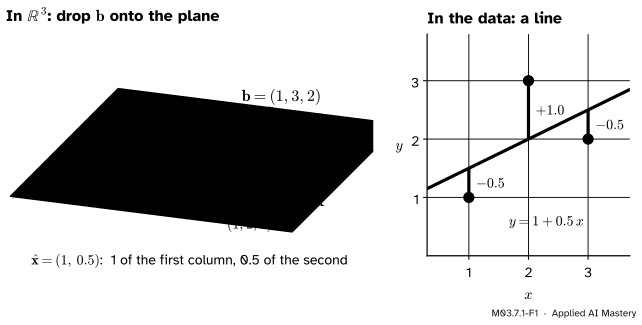
The same numbers can be read in two pictures. In the data picture they are three points and a line, and the misses are vertical gaps. In the second picture the three heights are one vector\(\vect{b} = (1, 3, 2)\) in \(\R^3\), with one axis per data point. Every choice of \(c\) and \(m\) gives a vector \(\mat{A}\vect{x} = c\,(1, 1, 1) + m\,(1, 2, 3)\), and all of those lie on one plane through the origin: the column space of \(\mat{A}\) (M02.7). The vector \(\vect{b}\) sticks out of that plane, which is why there is no exact solution.
M03.7.1-F1
One fit, two pictures. On the left, \(\vect{b}\) is dropped straight onto the plane of the columns; the foot of the drop is \(\mat{A}\hat{\vect{x}}\) and the drop itself is the residual \(\vect{e}\). On the right, the entries of \(\vect{e}\) are the vertical gaps between the points and the line.
Least squares asks for the \(\hat{\vect{x}}\) that makes the residual \(\vect{e} = \vect{b} - \mat{A}\hat{\vect{x}}\) as short as possible. Its squared length is the sum of the squared gaps, so “shortest residual” and “least sum of squares” are the same request. In the left picture the answer is plain to see: the closest point of a plane is the foot of the perpendicular. The whole lesson is that one sentence, turned into algebra.
Build it up
Step 1. Every prediction lies on the plane.\(\mat{A}\vect{x}\) is a combination of the columns of \(\mat{A}\) with weights \(c\) and \(m\) (the column rule of M02.5), so as \(\vect{x}\) varies, \(\mat{A}\vect{x}\) runs over the whole column space and nowhere else.
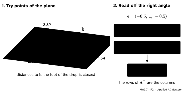
Step 2. Try some points of the plane. Measure the distance from \(\vect{b}\) to a few of them.
M03.7.1-F2
Every other point of the plane is farther from \(\vect{b}\) than the foot of the drop, and at the foot the residual is perpendicular to both columns. Two zero dot products are one matrix equation.
Step 3. The closest point is where the residual stands at a right angle. M02.10.4 proved this with Pythagoras: if \(\vect{e}\) is perpendicular to the plane and \(\vect{w}\) is any other point of the plane, then
Perpendicular to the plane means perpendicular to both columns, because every vector of the plane is a combination of them.
Step 4. Stack the right angles. Two dot products, written one above the other, are the rows of a matrix times \(\vect{e}\). The rows of that matrix are the columns of \(\mat{A}\), so it is \(\mat{A}\T\):
Let \(\mat{A}\) be \(m \times n\) and \(\vect{b}\) in \(\R^m\). A vector \(\hat{\vect{x}}\) minimises \(\norm{\vect{b} - \mat{A}\vect{x}}\) exactly when
If the columns of \(\mat{A}\) are independent, \(\mat{A}\T\mat{A}\) is invertible and \(\hat{\vect{x}} = {(\mat{A}\T\mat{A})^{-1}\mat{A}\T\vect{b}}\) is the only minimiser.
Derivation, in two lines. The best \(\hat{\vect{x}}\) makes the residual perpendicular to every column, which is \(\mat{A}\T\closs{\vect{e}} = \vect{0}\). Put in \(\vect{e} = \vect{b} - \mat{A}\hat{\vect{x}}\) and multiply out:
The steps run backwards too, so a solution of the normal equations makes \(\vect{e}\) perpendicular to the columns, and Step 3 shows it is a minimum. The same equations come out of setting the partial derivatives of the sum of squares to zero, the calculus route of ML01.4.3; here the geometry gives them without a derivative.
Why independent columns make \(\mat{A}\T\mat{A}\) invertible. Suppose \(\mat{A}\T\mat{A}\vect{v} = \vect{0}\). Multiply on the left by \(\vect{v}\T\):
So \(\mat{A}\vect{v} = \vect{0}\), and independent columns allow that only for \(\vect{v} = \vect{0}\). A square matrix that sends only \(\vect{0}\) to \(\vect{0}\) is invertible (M02.7).
The hat matrix. Put the formula for \(\hat{\vect{x}}\) into \(\mat{A}\hat{\vect{x}}\). The projection of \(\vect{b}\) is a fixed matrix times \(\vect{b}\):
Statisticians call \(\mat{H}\) the hat matrix, because it puts the hat on \(\vect{y}\). Three facts about it follow from the formula.
\(\mat{H}\) is symmetric. The transpose of a product is the product of the transposes in reverse order, and \(\mat{A}\T\mat{A}\) is symmetric, so its inverse is too:
In words: a point already on the plane stays put, so projecting twice is projecting once.
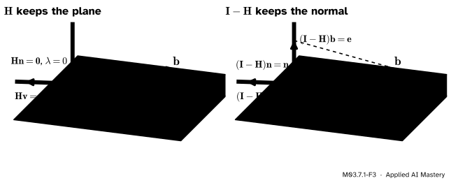
Its eigenvalues are only 0 and 1. If \(\mat{H}\vect{v} = \lambda\vect{v}\) with \(\vect{v} \ne \vect{0}\) (M03.1), then \({\lambda\vect{v}} = {\mat{H}\vect{v}} = {\mat{H}^2\vect{v}} = {\lambda^2\vect{v}}\), so \(\lambda^2 = \lambda\) and \(\lambda\) is 0 or 1. Every vector of the column space is an eigenvector for 1; every vector perpendicular to it, in the left null space \(N(\mat{A}\T)\), is an eigenvector for 0.
M03.7.1-F3
\(\mat{H}\) keeps every vector of the plane and flattens the direction at right angles to it, so its eigenvalues are 1 and 0. \(\mat{I} - \mat{H}\) does the opposite and returns the residual.
\(\mat{I} - \mat{H}\) projects onto the left null space. It sends \(\vect{b}\) to \(\vect{b} - \mat{H}\vect{b} = \vect{e}\), which lies in \(N(\mat{A}\T)\) because \(\mat{A}\T\vect{e} = \vect{0}\). It is symmetric, and \({(\mat{I} - \mat{H})^2} = {\mat{I} - 2\mat{H} + \mat{H}^2} = {\mat{I} - \mat{H}}\), so it is a projection too. Every \(\vect{b}\) splits into two perpendicular pieces, \(\vect{b} = {\mat{H}\vect{b}} + {(\mat{I} - \mat{H})\vect{b}}\): the part the model explains and the part it cannot.
Go deeper: the trace of H counts the columns
The trace of a matrix is the sum of its eigenvalues (M03.1). The eigenvalue 1 of \(\mat{H}\) has the column space as its eigenspace, of dimension \(n\) when the columns are independent, so \(\operatorname{tr}\mat{H} = n\). There is a one-line check through the rule \(\operatorname{tr}(\mat{X}\mat{Y}) = \operatorname{tr}(\mat{Y}\mat{X})\):
The diagonal entries \(h_{ii}\) are the leverages of the data points: how strongly each target pulls on its own fitted value. They add up to the number of parameters.
Worked example
The four running points \((0, 1)\), \((3, 2)\), \((4, 4)\), \((7, 5)\) of M02.10.4, by the normal equations. Here \(\mat{A}\) has a column of ones and the column \(\vect{x} = (0, 3, 4, 7)\), and \(\vect{b} = (1, 2, 4, 5)\).
M03.7.1-F4
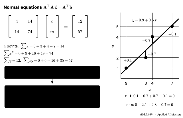
Every entry of \(\mat{A}\T\mat{A}\) and \(\mat{A}\T\vect{b}\) is a sum over the data. Solving the two-by-two system gives the line, and the residual passes the right-angle test against both columns.
Form the two sides. Each entry is a dot product of two columns: \(\vect{1} \cdot \vect{1} = 4\), \(\vect{1} \cdot \vect{x} = 14\), \(\vect{x} \cdot \vect{x} = 74\), \(\vect{1} \cdot \vect{b} = 12\) and \(\vect{x} \cdot \vect{b} = {0 + 6 + 16 + 35} = 57\). So
Solve. The determinant is \({4 \cdot 74} - {14^2} = {296 - 196} = 100\), and the inverse of a two-by-two matrix swaps the diagonal and negates the rest (M02.7):
This is the line \(y = 0.9 + 0.6\,x\) that QR found in M02.10.4, now with no Gram-Schmidt.
Check the right angle. The fitted values are \((0.9, 2.7, 3.3, 5.1)\), so \(\vect{e} = (0.1, -0.7, 0.7, -0.1)\). Against the column of ones the sum is \({0.1 - 0.7 + 0.7 - 0.1} = 0\); against \(\vect{x}\) it is \({0 - 2.1 + 2.8 - 0.7} = 0\). Both are zero, so \(\mat{A}\T\vect{e} = \vect{0}\), and the sum of squared gaps, \({0.01 + 0.49 + 0.49 + 0.01} = 1\), is the least possible.
Code
From scratch: form the normal equations, solve them, and build the hat matrix.
import numpy as npdef normal_equations(A, b):"""Least squares by A^T A x = A^T b (fine for small, well-behaved problems)."""return np.linalg.solve(A.T @ A, A.T @ b)def hat_matrix(A):"""H = A (A^T A)^{-1} A^T, the projection onto the column space of A."""return A @ np.linalg.solve(A.T @ A, A.T)x = np.array([0.0, 3.0, 4.0, 7.0])b = np.array([1.0, 2.0, 4.0, 5.0])A = np.column_stack([np.ones(4), x])x_hat = normal_equations(A, b)e = b - A @ x_hatH = hat_matrix(A)print("A^T A =\n", A.T @ A, "\nA^T b =", A.T @ b)print("x_hat =", x_hat, " residual e =", np.round(e, 10))print("A^T e =", np.round(A.T @ e, 12))print("H =\n", np.round(H, 2))print("eigenvalues of H:", np.round(np.linalg.eigvalsh(H), 10), " trace:", round(np.trace(H), 10))
A^T A =
 [[ 4. 14.]
 [14. 74.]]
A^T b = [12. 57.]
x_hat = [0.9 0.6]   residual e = [ 0.1 -0.7  0.7 -0.1]
A^T e = [-0.  0.]
H =
 [[ 0.74  0.32  0.18 -0.24]
 [ 0.32  0.26  0.24  0.18]
 [ 0.18  0.24  0.26  0.32]
 [-0.24  0.18  0.32  0.74]]
eigenvalues of H: [-0.  0.  1.  1.]   trace: 2.0
The eigenvalues come out as two zeros and two ones, up to rounding in the last digits, and the diagonal of \(\mat{H}\), the leverages \(0.74, 0.26, 0.26, 0.74\), adds up to 2. The outer points \(x = 0\) and \(x = 7\) pull hardest on the line. Now the three-point example of the opening, and the library call.
normal equations: [1.  0.5]   lstsq: [1.  0.5]   sum of squares: [1.5]
residual: [-0.5  1.  -0.5]   its length: 1.2247
numpy.linalg.lstsq returns the solution, the sum of squared residuals (\(1.5\) here, so \(\norm{\vect{e}} = \sqrt{1.5} \approx 1.22\)), the rank and the singular values. It does not form \(\mat{A}\T\mat{A}\) at all; the next lesson shows why that matters.
Explore
M03.7-X1
Least squares as projection
Set the three heights with the sliders, or drag the points in the lower panel. Turn the view to see that \(\vect{e}\) meets the plane at a right angle from every side. Then line the three points up exactly: what happens to \(\vect{b}\) and to \(\vect{e}\)?
Pitfalls
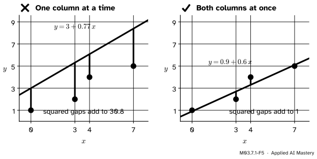
M03.7.1-F5
Wrong beside right. Fitting the constant alone gives \(c = 12/4 = 3\) and fitting the slope alone gives \(m = 57/74 \approx 0.77\), but the two shadows do not add up to the projection, because the columns \((1, 1, 1, 1)\) and \((0, 3, 4, 7)\) are not perpendicular.
“Project onto each column, then add the pieces.”
That works only when the columns are perpendicular, as with the orthonormal \(\vect{q}\)’s of M02.10.4. In general each column’s shadow already contains part of the other’s, so the pieces overlap. In machine learning this is the gap between fitting each feature on its own and fitting them together: the joint weights \(0.9\) and \(0.6\) are not the single-feature weights \(3\) and \(0.77\). The normal equations solve for all the weights at once.
“\((\mat{A}\T\mat{A})^{-1} = \mat{A}^{-1}(\mat{A}\T)^{-1}\), so \(\mat{H}\) is the identity.”
That rule needs square, invertible factors. A tall \(\mat{A}\) has no inverse, and \(\mat{H}\) is \(4 \times 4\) with rank 2. If \(\mat{H}\) were \(\mat{I}\), every target vector would already lie on the plane and every data set would sit exactly on a line. Only when \(\mat{A}\) is square and invertible does \(\mat{H} = \mat{I}\) hold.
“The residual is perpendicular to the fitted line in the data picture.”
The right angle lives in \(\R^m\), between \(\vect{e}\) and the columns of \(\mat{A}\). In the data picture the gaps are vertical, as M02.10.4 warned, and they meet the line at whatever angle its slope gives.
Check yourself
Recall
1. What condition on the residual picks out the least-squares solution?
Show answer
The residual \(\vect{e} = \vect{b} - \mat{A}\hat{\vect{x}}\) must be perpendicular to every column of \(\mat{A}\), that is \(\mat{A}\T\vect{e} = \vect{0}\).
3. When is \(\mat{A}\T\mat{A}\) invertible, and why?
Show answer
When the columns of \(\mat{A}\) are independent. If \(\mat{A}\T\mat{A}\vect{v} = \vect{0}\) then \({\norm{\mat{A}\vect{v}}^2} = {\vect{v}\T\mat{A}\T\mat{A}\vect{v}} = 0\), so \(\mat{A}\vect{v} = \vect{0}\), which forces \(\vect{v} = \vect{0}\).
4. Which two equations say that \(\mat{H}\) is a perpendicular projection?
Show answer
\(\mat{H}^2 = \mat{H}\) (projecting twice changes nothing) and \(\mat{H}\T = \mat{H}\) (it is symmetric).
5. What are the eigenvalues of the hat matrix, and what are their eigenvectors?
Show answer
Only 1 and 0. The vectors of the column space are eigenvectors for 1; the vectors of the left null space \(N(\mat{A}\T)\) are eigenvectors for 0.
Exercises
1.★ Write the normal equations for the three points \((1, 1)\), \((2, 3)\), \((3, 2)\) of the opening, solve them, and check that the residual is perpendicular to both columns.
Show solution
The columns are \(\vect{1} = (1, 1, 1)\) and \(\vect{x} = (1, 2, 3)\), and \(\vect{b} = (1, 3, 2)\). The entries are \(\vect{1} \cdot \vect{1} = 3\), \(\vect{1} \cdot \vect{x} = 6\), \(\vect{x} \cdot \vect{x} = 14\), \(\vect{1} \cdot \vect{b} = 6\) and \(\vect{x} \cdot \vect{b} = {1 + 6 + 6} = 13\):
The determinant is \({42 - 36} = 6\), so \(c = {(14 \cdot 6 - 6 \cdot 13)/6} = {6/6} = 1\) and \(m = {(-6 \cdot 6 + 3 \cdot 13)/6} = {3/6} = 0.5\). The fitted values are \((1.5, 2, 2.5)\) and \(\vect{e} = (-0.5, 1, -0.5)\). Then \({-0.5 + 1 - 0.5} = 0\) and \({-0.5 + 2 - 1.5} = 0\).
2.★★ Let \(\mat{A}\) have a single column \(\vect{a}\). Show that \(\mat{H} = \vect{a}\vect{a}\T / (\vect{a}\T\vect{a})\). Then take \(\vect{a} = (1, 1, 1, 1)\) and show that \(\mat{H}\vect{b}\) replaces every entry of \(\vect{b}\) by the mean of the entries.
Show solution
Here \(\mat{A}\T\mat{A} = \vect{a}\T\vect{a}\) is a single number, so its inverse is \(1/(\vect{a}\T\vect{a})\) and \(\mat{H} = {\vect{a}\,\tfrac{1}{\vect{a}\T\vect{a}}\,\vect{a}\T} = {\vect{a}\vect{a}\T/(\vect{a}\T\vect{a})}\), the projection onto a line of M02.3. For \(\vect{a} = (1, 1, 1, 1)\), \(\vect{a}\T\vect{a} = 4\) and \(\vect{a}\T\vect{b} = b_1 + b_2 + b_3 + b_4\), so
a vector whose entries all equal the mean \(\bar{b}\). Fitting a model that is only a constant gives the mean, which is why the mean is the least-squares summary of a list of numbers.
3.★★★ Prove that \(\operatorname{tr}\mat{H} = n\) when the \(n\) columns of \(\mat{A}\) are independent, using the fact that \(\mat{H}\) has only the eigenvalues 0 and 1. Check it on the four running points.
Show solution
\(\mat{H}\) is symmetric, so by the spectral theorem (M03.3) it has an orthonormal basis of eigenvectors and its trace is the sum of its eigenvalues, each 0 or 1. The number of ones is the dimension of the eigenspace for 1. A vector \(\vect{v}\) has \(\mat{H}\vect{v} = \vect{v}\) exactly when \(\vect{v}\) is in the column space: if \(\vect{v} = \mat{A}\vect{z}\) then \(\mat{H}\vect{v} = {\mat{A}(\mat{A}\T\mat{A})^{-1}\mat{A}\T\mat{A}\vect{z}} = \mat{A}\vect{z} = \vect{v}\), and conversely \(\mat{H}\vect{v}\) always lies in the column space. With independent columns that space has dimension \(n\), so \(\operatorname{tr}\mat{H} = n\). For the four points the diagonal is \((0.74, 0.26, 0.26, 0.74)\), with sum \(2\), the number of columns.
Summary card
Least squares drops \(\vect{b}\) straight onto the column space.
M03.7.1-F1
One right angle, two pictures.
Right angle.\(\mat{A}\T\vect{e} = \vect{0}\) for \(\vect{e} = \vect{b} - \mat{A}\hat{\vect{x}}\).
Normal equations.\(\mat{A}\T\mat{A}\,\hat{\vect{x}} = \mat{A}\T\vect{b}\).
Hat matrix.\(\mat{H} = \mat{A}(\mat{A}\T\mat{A})^{-1}\mat{A}\T\) with \(\mat{H}^2 = \mat{H} = \mat{H}\T\).
Sources. Each was opened and checked against this lesson on 15 November 2026.
Gilbert Strang, Projection matrices and least squares, MIT OpenCourseWare 18.06SC, lecture 16 and its lecture summary. The summary gives \(\mat{P} = \mat{A}(\mat{A}\T\mat{A})^{-1}\mat{A}\T\), says that \(\mat{I} - \mat{P}\) projects onto \(N(\mat{A}\T)\), and reads a three-point line fit in the same two views as this lesson: vertical gaps in the data, and \(\vect{b}\) in \(\R^3\) projected onto the column space.
Dan Margalit and Joseph Rabinoff, Interactive Linear Algebra, Section 6.5. The theorem that the least-squares solutions of \(\mat{A}\vect{x} = \vect{b}\) are the solutions of \(\mat{A}\T\mat{A}\vect{x} = \mat{A}\T\vect{b}\), and the theorem that a unique solution, independent columns and an invertible \(\mat{A}\T\mat{A}\) are equivalent.