The SVD of a tall or wide matrix: the shapes of the full and the thin factorisation, the rank as the number of non-zero singular values, and orthonormal bases of all four fundamental subspaces read straight off the columns of U and V.
M03.5.3L2 Intermediate25 minIn review (what this means)
The maths and code on this page are checked by automated tests on every change, but an independent reader has not signed it off yet. Spot a mistake or a confusing step? Tell us.
Give the shapes of U, Sigma and V in the full and the thin SVD of an m by n matrix, and explain why the thin one loses nothing.
Compute the SVD of a 3 by 2 matrix by hand, including a basis of its left null space.
Prove that the first r columns of U and V span the column space and the row space, and the rest span the left null space and the null space.
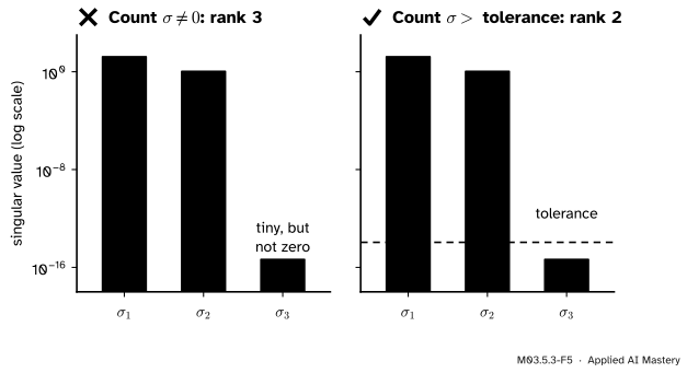
Find the rank as the number of singular values above a tolerance, and explain why counting non-zero values fails in floating point.
The question
A data matrix is rarely square: a thousand customers by twenty features, or ten thousand words by three hundred documents. Such a matrix maps one space into a space of a different size. What does its SVD look like, and how does it tell us which outputs can be reached at all, and which inputs are lost without trace?
From the last lesson
1. How are the singular values of \(\mat{A}\) related to the eigenvalues of \(\mat{A}\T\mat{A}\)?
Show answer
\(\sigma_i = \sqrt{\lambda_i}\): the singular values are the non-negative square roots of the eigenvalues of \(\mat{A}\T\mat{A}\), and its eigenvectors are the \(\vect{v}_i\).
2. Once \(\vect{v}_i\) and \(\sigma_i > 0\) are known, how do you find \(\vect{u}_i\), and why that way rather than from \(\mat{A}\mat{A}\T\)?
Show answer
\(\vect{u}_i = \mat{A}\vect{v}_i/\sigma_i\). Found separately from \(\mat{A}\mat{A}\T\), an eigenvector could come out with the wrong sign, and then \(\mat{U}\mat{\Sigma}\mat{V}\T \ne \mat{A}\).
Intuition
Take the running rectangular matrix of this course,
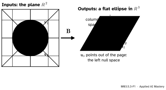
which sends the plane \(\R^2\) into space \(\R^3\). The unit circle still goes to an ellipse, but now the ellipse is flat and floats in space. It lies in a plane through the origin: the column space of \(\mat{B}\), everything that \(\mat{B}\) can reach (M02.7.2).
M03.5.3-F1
\(\mat{B}\) sends the unit circle to a flat ellipse inside its column space. The SVD supplies two perpendicular axes of that ellipse and a third direction, \(\vect{u}_3\), straight out of the plane, that no input ever reaches.
The SVD still finds perpendicular inputs \(\vect{v}_1, \vect{v}_2\) that land on the axes, \(\sigma_1\vect{u}_1\) and \(\sigma_2\vect{u}_2\). But space has a third direction. The unit vector \(\vect{u}_3\), perpendicular to the plane, completes the set. Nothing lands on it: it spans the left null space. One factorisation hands us both what the matrix reaches and what it misses.
Build it up
Step 1. The shapes. For an \(m\) by \(n\) matrix the SVD is still \(\mat{A} = \mat{U}\mat{\Sigma}\mat{V}\T\), but the three factors have different shapes:
\(\mat{V}\) is \(n\) by \(n\), orthogonal: an orthonormal basis of the input space \(\R^n\).
\(\mat{U}\) is \(m\) by \(m\), orthogonal: an orthonormal basis of the output space \(\R^m\).
\(\mat{\Sigma}\) is \(m\) by \(n\), the same shape as \(\mat{A}\), with \(\sigma_1, \sigma_2, \dots\) down its diagonal and zeros everywhere else.
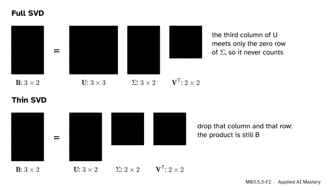
For \(\mat{B}\) that is \({3 \times 2} = {(3 \times 3)(3 \times 2)(2 \times 2)}\). The third row of \(\mat{\Sigma}\) is all zeros.
Step 2. The thin SVD. In the product \(\mat{U}\mat{\Sigma}\), column 3 of \(\mat{U}\) is multiplied only by row 3 of \(\mat{\Sigma}\), which is zero. So delete both. What is left, \(\mat{U}\) with two columns and a square 2 by 2 \(\mat{\Sigma}\), multiplies out to the same \(\mat{B}\). This is the thin SVD: with \(k = \min(m, n)\), \(\mat{U}\) is \({m \times k}\), \(\mat{\Sigma}\) is \({k \times k}\) and \(\mat{V}\T\) is \({k \times n}\). NumPy gives the full one by default and the thin one with full_matrices=False.
M03.5.3-F2
The full and the thin SVD of the 3 by 2 matrix \(\mat{B}\). The column of \(\mat{U}\) that meets the zero row of \(\mat{\Sigma}\) contributes nothing to the product.
Step 3. The rank. Some singular values may be zero, even when the matrix is square. The number \(r\) of non-zero singular values is the rank, as we prove next. The first \(r\) columns of \(\mat{U}\) and \(\mat{V}\) do all the work; the rest describe what is missed.
The formal statement
NoteTheorem: the SVD and the four fundamental subspaces
Let \(\mat{A} = \mat{U}\mat{\Sigma}\mat{V}\T\) be an \(m\) by \(n\) matrix with exactly \(r\) positive singular values. Then
\(\vect{u}_1, \dots, \vect{u}_r\) is an orthonormal basis of the column space;
\(\vect{u}_{r+1}, \dots, \vect{u}_m\) is an orthonormal basis of the left null space;
\(\vect{v}_1, \dots, \vect{v}_r\) is an orthonormal basis of the row space;
\(\vect{v}_{r+1}, \dots, \vect{v}_n\) is an orthonormal basis of the null space;
and the rank of \(\mat{A}\) is \(r\).
Proof. Every input is a combination of the orthonormal basis \(\vect{v}_1, \dots, \vect{v}_n\): \(\vect{x} = {c_1\vect{v}_1 + \dots + c_n\vect{v}_n}\) with \(c_i = {\vect{v}_i \cdot \vect{x}}\). Apply \(\mat{A}\), using \(\mat{A}\vect{v}_i = \sigma_i\vect{u}_i\) for \(i \le r\) and \(\mat{A}\vect{v}_i = \vect{0}\) for \(i > r\):
Column space. Every output is therefore a combination of \(\vect{u}_1, \dots, \vect{u}_r\), and each \(\vect{u}_i\) is reached, by the input \(\vect{v}_i/\sigma_i\). So the column space is exactly their span. They are orthonormal, hence independent, so its dimension, the rank, is \(r\).
Null space.\(\mat{A}\vect{x} = \vect{0}\) exactly when every coefficient \(c_i\sigma_i\) with \(i \le r\) is zero, because the \(\vect{u}_i\) are independent. Since \(\sigma_i > 0\), that means \(c_1 = \dots = c_r = 0\), so \(\vect{x}\) is a combination of \(\vect{v}_{r+1}, \dots, \vect{v}_n\).
Row space and left null space. M02.7.4 showed that the row space is the set of vectors perpendicular to the null space, and the left null space the set perpendicular to the column space. The vectors perpendicular to \(\vect{v}_{r+1}, \dots, \vect{v}_n\) are the combinations of the other \(\vect{v}\)’s, and likewise for the \(\vect{u}\)’s. \(\blacksquare\)
The counting rule of M02.7.4 drops out: the null space has \(n - r\) basis vectors and the left null space \(m - r\). And the SVD says more than the rule: it gives perpendicular bases, and it pairs them, \(\vect{v}_i\) in the row space with \(\vect{u}_i\) in the column space.
M03.5.3-F3
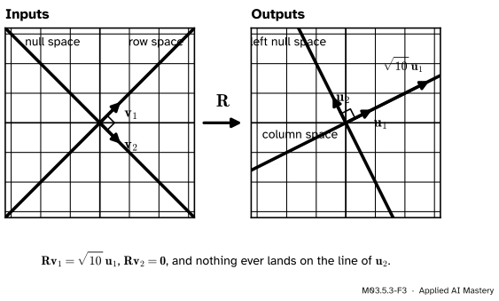
The four subspaces of the rank-one matrix \(\mat{R}\), with rows \((2, 2)\) and \((1, 1)\). Its one non-zero singular value is \(\sqrt{10}\).
For this \(\mat{R}\), \(\mat{R}\T\mat{R}\) has rows \((5, 5)\) twice, with eigenvalues \(10\) and \(0\). So \(\sigma_1 = \sqrt{10}\), \(\sigma_2 = 0\) and the rank is \(1\). The row space is the line of \(\vect{v}_1 = (1, 1)/\sqrt{2}\) and the null space the line of \(\vect{v}_2 = (1, -1)/\sqrt{2}\). Then \(\mat{R}\vect{v}_1 = {(4, 2)/\sqrt{2}}\), of length \(\sqrt{10}\), so \(\vect{u}_1 = (2, 1)/\sqrt{5}\) spans the column space, and the perpendicular \(\vect{u}_2 = (-1, 2)/\sqrt{5}\) spans the left null space. Four lines, two right angles: the picture of M02.7.4, now with unit vectors on every line.
Worked example
Find the full SVD of \(\mat{B}\), and all four of its subspaces.
Step 1. The entries of \(\mat{B}\T\mat{B}\) are dot products of the columns \((1, 1, 0)\) and \((1, 0, 1)\): \(1 + 1 + 0 = 2\), \(1 + 0 + 0 = 1\) and \(1 + 0 + 1 = 2\). So \(\mat{B}\T\mat{B}\) is the running symmetric matrix \(\mat{S}\) of M03.3, with rows \((2, 1)\) and \((1, 2)\).
Step 2. Its trace is \(4\) and its determinant \(3\), so \(\lambda^2 - 4\lambda + 3 = {(\lambda - 3)(\lambda - 1)}\): eigenvalues \(3\) and \(1\), with eigenvectors \(\vect{v}_1 = (1, 1)/\sqrt{2}\) and \(\vect{v}_2 = (1, -1)/\sqrt{2}\). So \(\sigma_1 = \sqrt{3}\) and \(\sigma_2 = 1\).
For \(\vect{u}_1\) we divided by \(\sqrt{3}\), using \({\sqrt{2}\,\sqrt{3}} = \sqrt{6}\); for \(\vect{u}_2\) by \(1\).
Step 4. The third column of \(\mat{U}\) must be a unit vector perpendicular to the column space, which is the left null space: all \(\vect{y}\) with \(\mat{B}\T\vect{y} = \vect{0}\). The rows of \(\mat{B}\T\) give \(y_1 + y_2 = 0\) and \(y_1 + y_3 = 0\), so \(\vect{y} = {y_1(1, -1, -1)}\) and
The four subspaces. The rank is \(r = 2\). Row space: all of \(\R^2\), spanned by \(\vect{v}_1, \vect{v}_2\). Null space: only \(\vect{0}\), since \(n - r = 0\). Column space: the plane spanned by \(\vect{u}_1\) and \(\vect{u}_2\). Left null space: the line of \(\vect{u}_3\), of dimension \(m - r = 1\).
M03.5.3-F4
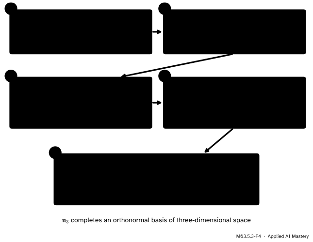
The worked example as a trace. Steps 1 to 4 are the recipe of lesson M03.5.2; step 5 completes \(\mat{U}\) with the left null space.
Code
The full and the thin SVD of \(\mat{B}\) from NumPy, with their shapes, and the four subspaces read off them.
import numpy as npB = np.array([[1.0, 1.0], [1.0, 0.0], [0.0, 1.0]])U, s, Vh = np.linalg.svd(B) # full_matrices=True is the defaultUt, st, Vht = np.linalg.svd(B, full_matrices=False)print("full:", U.shape, s.shape, Vh.shape, " thin:", Ut.shape, st.shape, Vht.shape)print("singular values:", s)Sigma = np.zeros((3, 2)) # the full Sigma has the shape of BSigma[:2, :2] = np.diag(s)print("full product equals B:", np.allclose(U @ Sigma @ Vh, B))print("thin product equals B:", np.allclose(Ut @ np.diag(st) @ Vht, B))print("third column of U:", np.round(U[:, 2], 4), " B^T times it:", np.round(B.T @ U[:, 2], 12) +0.0)
full: (3, 3) (2,) (2, 2)   thin: (3, 2) (2,) (2, 2)
singular values: [1.73205081 1.        ]
full product equals B: True
thin product equals B: True
third column of U: [-0.5774  0.5774  0.5774]   B^T times it: [0. 0.]
The rank is the number of singular values that are not zero. In floating point “not zero” needs a tolerance. The matrix with rows \((1, 2, 3)\), \((4, 5, 6)\), \((7, 8, 9)\) has rank 2 (its third row minus its second equals its second minus its first), but its computed third singular value is typically a tiny number near \(10^{-16}\) rather than an exact zero. NumPy’s matrix_rank counts the singular values above \(\sigma_1 \cdot \max(m, n) \cdot \varepsilon\), where \(\varepsilon\) is the spacing of double-precision numbers near 1.
M = np.array([[1.0, 2.0, 3.0], [4.0, 5.0, 6.0], [7.0, 8.0, 9.0]])sM = np.linalg.svd(M, compute_uv=False)tol = sM.max() *max(M.shape) * np.finfo(float).epsprint("singular values:", sM)print("tolerance:", tol)print("rank by tolerance:", int(np.sum(sM > tol)), " numpy.linalg.matrix_rank:", np.linalg.matrix_rank(M))# The four subspaces of the rank-one matrix R, read off its full SVD.R = np.array([[2.0, 2.0], [1.0, 1.0]])UR, sR, VhR = np.linalg.svd(R)r =int(np.sum(sR > sR.max() *2* np.finfo(float).eps))print("R: sigma =", np.round(sR, 6), " rank", r)print("null space basis:", np.round(VhR[r:], 4), " left null space basis:", np.round(UR[:, r:].T, 4))
singular values: [1.68481034e+01 1.06836951e+00 3.35890790e-16]
tolerance: 1.1223091358001953e-14
rank by tolerance: 2   numpy.linalg.matrix_rank: 2
R: sigma = [3.162278 0.      ]  rank 1
null space basis: [[ 0.7071 -0.7071]]   left null space basis: [[-0.4472  0.8944]]
Explore
The module’s interactive, Rotate, stretch, rotate, is in lesson M03.5.1. Choose the preset “Rank 1” or drag \(\mat{A}\jhat\) onto the line of \(\mat{A}\ihat\): the ellipse collapses to a segment, \(\sigma_2\) becomes \(0\), and the read-out reports rank 1. The segment is the column space; the line perpendicular to it is the left null space.
Pitfalls
M03.5.3-F5
Wrong beside right. Rounding leaves a tiny third singular value, so counting non-zero values gives rank 3; counting those above a tolerance gives the true rank, 2.
“The rank is the number of singular values that are not zero, so I count them.”
In exact arithmetic, yes. In floating point a singular value that should be zero comes out as rounding noise, perhaps \(10^{-16}\). Count the singular values above a tolerance, as numpy.linalg.matrix_rank does. Choosing that tolerance is a judgement about the data: with noisy measurements, a singular value of \(10^{-6}\) may be noise too (M03.6 and M03.7.4 return to this).
“The thin \(\mat{U}\) has orthonormal columns, so \(\mat{U}\mat{U}\T = \mat{I}\).”
Only \(\mat{U}\T\mat{U} = \mat{I}\), the 2 by 2 identity, holds: it compares the columns with each other. The 3 by 3 product \(\mat{U}\mat{U}\T\) is not the identity. It is \({\vect{u}_1\vect{u}_1\T + \vect{u}_2\vect{u}_2\T}\), the projection onto the column space, and it sends \(\vect{u}_3\) to \(\vect{0}\). Lesson M03.7.1 meets it again as the hat matrix.
“The extra columns of the full \(\mat{U}\) are determined by \(\mat{A}\).”
They are any orthonormal basis of the left null space. When that space has dimension 2 or more, there are infinitely many choices, and different libraries may return different ones. Nothing in \(\mat{A} = \mat{U}\mat{\Sigma}\mat{V}\T\) depends on the choice, because those columns meet zeros.
Check yourself
Recall
1. What are the shapes of \(\mat{U}\), \(\mat{\Sigma}\) and \(\mat{V}\) in the full SVD of an \(m\) by \(n\) matrix?
Show answer
\(\mat{U}\) is \({m \times m}\), \(\mat{\Sigma}\) is \({m \times n}\) and \(\mat{V}\) is \({n \times n}\).
2. How do you read the rank off the SVD?
Show answer
It is the number of positive singular values; in floating point, the number above a tolerance.
3. Which columns of \(\mat{U}\) span the left null space?
Show answer
\(\vect{u}_{r+1}, \dots, \vect{u}_m\), the columns beyond the rank.
4. What are the singular values of \(\mat{B}\), with rows \((1, 1)\), \((1, 0)\), \((0, 1)\)?
Show answer
\(\sqrt{3}\) and \(1\), the square roots of the eigenvalues \(3\) and \(1\) of \(\mat{B}\T\mat{B} = \mat{S}\).
5. Why does the thin SVD give the same product as the full one?
Show answer
The columns of \(\mat{U}\) that are dropped are multiplied only by the zero rows of \(\mat{\Sigma}\), so they contribute nothing.
Exercises
1.★ A data matrix \(\mat{X}\) is 100 by 5 with rank 5. Give the shapes of the three factors in its full and thin SVD, and the dimensions of its four subspaces. Do the same for \(\mat{X}\T\).
Show solution
\(\mat{X}\): full \(\mat{U}\) is \({100 \times 100}\), \(\mat{\Sigma}\) is \({100 \times 5}\), \(\mat{V}\T\) is \({5 \times 5}\); thin \(\mat{U}\) is \({100 \times 5}\), \(\mat{\Sigma}\) is \({5 \times 5}\), \(\mat{V}\T\) is \({5 \times 5}\). Row space dimension 5, null space \(0\), column space \(5\), left null space \({100 - 5} = 95\). \(\mat{X}\T\) is \({5 \times 100}\): full \(\mat{U}\) is \({5 \times 5}\), \(\mat{\Sigma}\) is \({5 \times 100}\), \(\mat{V}\T\) is \({100 \times 100}\); thin \(\mat{U}\) is \({5 \times 5}\), \(\mat{\Sigma}\) is \({5 \times 5}\), \(\mat{V}\T\) is \({5 \times 100}\). Its row space has dimension 5, its null space 95, its column space 5 and its left null space 0.
2.★★ Write down an SVD of \(\mat{B}\T\), the 2 by 3 matrix with rows \((1, 1, 0)\) and \((1, 0, 1)\), using the SVD of \(\mat{B}\) found above. What is its null space?
Show solution
Transposing \(\mat{B} = \mat{U}\mat{\Sigma}\mat{V}\T\) gives \(\mat{B}\T = \mat{V}\mat{\Sigma}\T\mat{U}\T\), which is again an SVD: \(\mat{V}\) and \(\mat{U}\) are orthogonal and \(\mat{\Sigma}\T\) is 2 by 3 with \(\sqrt{3}\) and \(1\) on its diagonal. So the roles swap: the right singular vectors of \(\mat{B}\T\) are \(\vect{u}_1, \vect{u}_2, \vect{u}_3\), the left ones are \(\vect{v}_1, \vect{v}_2\), and \(\mat{B}\T\vect{u}_1 = \sqrt{3}\,\vect{v}_1\), \(\mat{B}\T\vect{u}_2 = \vect{v}_2\), \(\mat{B}\T\vect{u}_3 = \vect{0}\). The null space of \(\mat{B}\T\) is the line of \(\vect{u}_3 = (1, -1, -1)/\sqrt{3}\), which is the left null space of \(\mat{B}\), as the name says.
3.★★★ Let \(\mat{A}\) have rank \(r\). Prove that for every \(\vect{x}\) in the row space, \({\norm{\mat{A}\vect{x}} \ge \sigma_r\norm{\vect{x}}}\), and conclude that \(\mat{A}\) sends different row-space vectors to different outputs.
Show solution
A row-space vector is \(\vect{x} = {c_1\vect{v}_1 + \dots + c_r\vect{v}_r}\), so \(\norm{\vect{x}}^2 = {c_1^2 + \dots + c_r^2}\) and \(\mat{A}\vect{x} = {c_1\sigma_1\vect{u}_1 + \dots + c_r\sigma_r\vect{u}_r}\). The \(\vect{u}_i\) are orthonormal, so
because every \(\sigma_i \ge \sigma_r\). If two row-space vectors \(\vect{x}\) and \(\vect{y}\) had the same output, their difference, which is in the row space, would satisfy \({0 = \norm{\mat{A}(\vect{x} - \vect{y})}} \ge \sigma_r\norm{\vect{x} - \vect{y}}\). Since \(\sigma_r > 0\), \(\vect{x} = \vect{y}\). So \(\mat{A}\) maps its row space one-to-one onto its column space; everything it destroys lies in the null space.
Summary card
The columns of \(\mat{U}\) and \(\mat{V}\) are orthonormal bases of all four fundamental subspaces, split at the rank \(r\).
Sources. Each was opened and checked against this lesson on 15 November 2026.
David Austin, Understanding Linear Algebra, section “Singular value decompositions”: the number of non-zero singular values is the rank; the first \(r\) left singular vectors span the column space and the rest the null space of the transpose; the first \(r\) right singular vectors span the row space and the rest the null space; the reduced SVD \(\mat{U}_r\mat{\Sigma}_r\mat{V}_r\T\).
Sheldon Axler, Linear Algebra Done Right, 4th edition, Section 7E: 7.68 (the number of positive singular values equals the dimension of the range) and 7.80 (the matrix SVD of a \(p\) by \(n\) matrix of rank \(m\) with \({p \times m}\) and \({n \times m}\) factors with orthonormal columns: the thin SVD with the zero singular values dropped as well).
Gilbert Strang, Singular value decomposition, MIT OpenCourseWare 18.06SC, lecture 29: the columns of \(\mat{U}\) and \(\mat{V}\) give bases for the four fundamental subspaces.