The eigenvalues add up to the trace and multiply to the determinant. See why, collect the eigenvectors of one eigenvalue into a subspace, tell a repeated eigenvalue with a plane of eigenvectors from one with a single line, and prove that different eigenvalues give independent eigenvectors.
M03.1.3L2 Intermediate25 minIn review (what this means)
The maths and code on this page are checked by automated tests on every change, but an independent reader has not signed it off yet. Spot a mistake or a confusing step? Tell us.
Derive that the eigenvalues of a 2 by 2 matrix sum to its trace and multiply to its determinant, and use both facts to check an answer.
Find the eigenspace of an eigenvalue and compare its algebraic and geometric multiplicity, on the identity and the shear.
Prove that eigenvectors for different eigenvalues are linearly independent.
Derive the eigenvalues of A to the power k, of A inverse and of A + cI, and show that similar matrices share their eigenvalues.
The question
A covariance matrix has the variances of the features on its diagonal, so its trace is the total variance of the data. Principal component analysis splits that total into the variances along its eigenvectors. Why do the eigenvalues add up to exactly the trace, and what else can be read off them without solving anything?
From the last lesson
1. Write the characteristic polynomial of a 2 by 2 matrix in terms of its trace and determinant.
2. Once you have an eigenvalue, how do you find its eigenvectors?
Show answer
Solve \({(\mat{A} - \lambda\mat{I})\vect{v}} = \vect{0}\) by elimination; the eigenvectors are the non-zero vectors of that null space.
Intuition
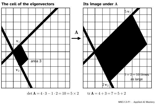
The determinant is the factor by which a matrix scales area (M02.8). Measure that area on the parallelogram built from two eigenvectors. Each side stays on its own line and is stretched by its own eigenvalue, so the area is multiplied by both.
M03.1.3-F1
Along its eigenvectors \(\mat{A}\) stretches one side 5 times and the other 2 times, so the cell they span, and every other area, grows \({5 \times 2} = 10\) times. That is \(\det\mat{A}\). The eigenvalues also add up to the trace, \({4 + 3} = {5 + 2}\).
The product rule needs only the picture. The sum rule needs one line of algebra, which follows.
Build it up
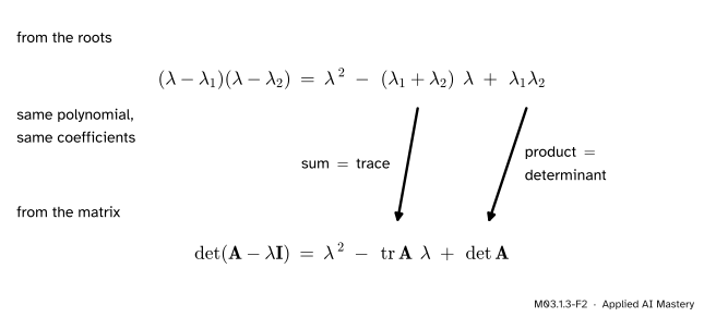
Step 1. Two ways to write one polynomial. If \(\lambda_1\) and \(\lambda_2\) are the roots of the characteristic polynomial, it factors as \({(\lambda - \lambda_1)(\lambda - \lambda_2)}\), because a quadratic with leading coefficient 1 is fixed by its roots. Multiplying out:
Last lesson the same polynomial came out as \({\lambda^2 - \operatorname{tr}(\mat{A})\,\lambda + \det\mat{A}}\).
M03.1.3-F2
The same polynomial written twice. Matching the coefficients of \(\lambda\) gives “sum of eigenvalues equals trace”, and matching the constants gives “product equals determinant”.
Step 2. Match the coefficients. Two polynomials that are equal for every \(\lambda\) have equal coefficients. So
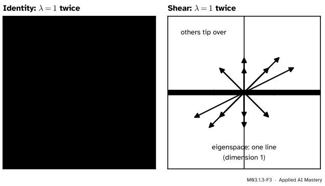
Step 3. A repeated root. When \(\lambda_1 = \lambda_2\) the eigenvalue is counted twice. The identity \(\mat{I}\) and the shear\(\begin{bmatrix} 1 & 1 \\ 0 & 1 \end{bmatrix}\) both have characteristic polynomial \({(\lambda - 1)^2}\): trace 2, determinant 1. Yet they behave very differently.
M03.1.3-F3
The same repeated eigenvalue, two different stories. The identity keeps every vector, so its eigenvectors fill the plane. The shear keeps only the horizontal line.
For the identity, \({(\mat{I} - 1\mat{I})\vect{v}} = \vect{0}\) for every \(\vect{v}\), so every non-zero vector is an eigenvector. For the shear, \(\mat{A} - \mat{I}\) has rows \((0, 1)\) and \((0, 0)\), which says \(y = 0\): only the horizontal line.
The formal statement
NoteTheorem: sum and product of the eigenvalues
Let \(\mat{A}\) be \({n \times n}\) with eigenvalues \({\lambda_1, \dots, \lambda_n}\), listed with repeats and including complex ones. Then
Steps 1 and 2 proved it for \(n = 2\). For larger \(n\), the polynomial \({\det(\mat{A} - \lambda\mat{I})}\) has degree \(n\) and leading term \({(-1)^n\lambda^n}\), so over the complex numbers it factors completely as \({(\lambda_1 - \lambda)(\lambda_2 - \lambda) \cdots (\lambda_n - \lambda)}\). Putting \(\lambda = 0\) on both sides gives \({\det\mat{A}} = {\lambda_1 \cdots \lambda_n}\).
Go deeper: the trace for n by n
In the factored form, the coefficient of \(\lambda^{n-1}\) is \({(-1)^{n-1}(\lambda_1 + \cdots + \lambda_n)}\): choose \(-\lambda\) from all but one bracket and the root from the remaining one. In the determinant, a term with \(n - 1\) factors of \(\lambda\) must use \(n - 1\) diagonal entries, and a permutation that fixes \(n - 1\) places fixes the last one too. So only the diagonal product contributes, and its \(\lambda^{n-1}\) coefficient is \({(-1)^{n-1}(a_{11} + \cdots + a_{nn})}\). Equating the two gives the trace rule.
Eigenspaces. For an eigenvalue \(\lambda\), the eigenspace\(E_\lambda\) is the null space of \(\mat{A} - \lambda\mat{I}\): all the eigenvectors for \(\lambda\) together with \(\vect{0}\). It is a subspace: if \({\mat{A}\vect{u}} = {\lambda\vect{u}}\) and \({\mat{A}\vect{w}} = {\lambda\vect{w}}\), then
The algebraic multiplicity of \(\lambda\) is the number of times it is a root of the characteristic polynomial. The geometric multiplicity is the dimension of \(E_\lambda\). The geometric multiplicity is always at least 1 and at most the algebraic one. The identity has 2 and 2; the shear has algebraic 2 but geometric 1, and such a matrix is called defective.
NoteTheorem: different eigenvalues, independent eigenvectors
Eigenvectors that belong to different eigenvalues are linearly independent.
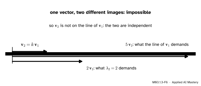
Proof for two. Let \({\mat{A}\vect{v}_1} = {\lambda_1\vect{v}_1}\) and \({\mat{A}\vect{v}_2} = {\lambda_2\vect{v}_2}\) with \(\lambda_1 \neq \lambda_2\), and suppose \({c_1\vect{v}_1 + c_2\vect{v}_2} = \vect{0}\). Apply \(\mat{A}\), and separately multiply by \(\lambda_2\):
Subtract the second line from the first: \({c_1(\lambda_1 - \lambda_2)\vect{v}_1} = \vect{0}\). Since \(\lambda_1 \neq \lambda_2\) and \(\vect{v}_1 \neq \vect{0}\), \(c_1 = 0\). Then \({c_2\vect{v}_2} = \vect{0}\) gives \(c_2 = 0\). Only the trivial combination is zero, so the two are independent. \(\blacksquare\)
M03.1.3-F6
The proof as a picture. If \(\vect{v}_2\) lay on the line of \(\vect{v}_1\), the matrix would have to stretch it by \(\lambda_1\) and by \(\lambda_2\) at once.
Go deeper: the induction for any number of eigenvectors
Suppose some list of eigenvectors with distinct eigenvalues is dependent, and take a shortest such list \({\vect{v}_1, \dots, \vect{v}_m}\), with \({a_1\vect{v}_1 + \cdots + a_m\vect{v}_m} = \vect{0}\). Here \({m \ge 2}\), because a single eigenvector is non-zero and so independent on its own. Every \(a_i\) is non-zero, or a shorter list would do. Apply \({\mat{A} - \lambda_m\mat{I}}\): each \(\vect{v}_i\) becomes \({(\lambda_i - \lambda_m)\vect{v}_i}\), and the last term vanishes, leaving
These coefficients are non-zero because the eigenvalues differ, so a shorter dependent list exists: a contradiction. This is Axler’s proof of result 5.11. In particular, an \({n \times n}\) matrix with \(n\) distinct eigenvalues has \(n\) independent eigenvectors, a basis of \(\R^n\); lesson M03.2.1 builds on exactly that.
Related matrices. If \({\mat{A}\vect{v}} = {\lambda\vect{v}}\), then for the same \(\vect{v}\):
Repeating the first step gives \({\mat{A}^k\vect{v}} = {\lambda^k\vect{v}}\) for every whole number \(k\). If \(\mat{A}\) is invertible, then \(\lambda \neq 0\) (a zero eigenvalue would crush \(\vect{v}\)), and multiplying \({\mat{A}\vect{v}} = {\lambda\vect{v}}\) by \(\mat{A}^{-1}\) and then by \(\frac{1}{\lambda}\) gives \({\mat{A}^{-1}\vect{v}} = {\frac{1}{\lambda}\vect{v}}\).
Similar matrices share eigenvalues. If \({\mat{B}} = {\mat{P}^{-1}\mat{A}\mat{P}}\) (lesson M02.9.3), write \(\mat{I} = {\mat{P}^{-1}\mat{I}\mat{P}}\) and use the product rule for determinants:
The last step uses \({\det(\mat{P}^{-1})\det\mat{P}} = {\det(\mat{P}^{-1}\mat{P})} = 1\). Same polynomial, same eigenvalues: the eigenvalues belong to the map, not to the basis it is written in. The eigenvectors do change, from \(\vect{v}\) to \(\mat{P}^{-1}\vect{v}\).
Worked example
Check the theorem on the running \(\mat{A}\), and find the eigenvalues of \(\mat{A}^2\), \(\mat{A}^{-1}\) and \(\mat{A} + 3\mat{I}\) without solving anything.
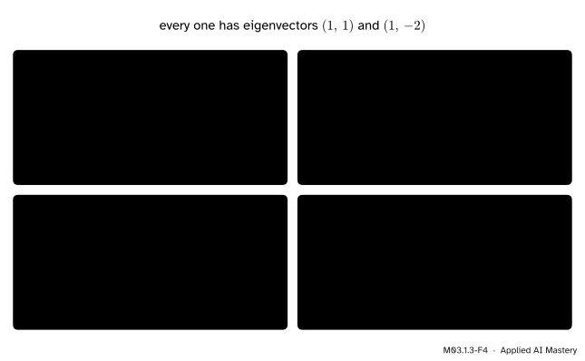
The related matrices. From the rules: \(\mat{A}^2\) has \(25\) and \(4\); \(\mat{A}^{-1}\) has \(\frac15\) and \(\frac12\); \(\mat{A} + 3\mat{I}\) has 8 and 5, all with the eigenvectors \((1, 1)\) and \((1, -2)\).
M03.1.3-F4
Each predicted pair of eigenvalues passes both checks against the actual matrix: the sum is its trace and the product its determinant.
Check them against the matrices themselves. Row times column gives
with trace \(0.7 = {0.2 + 0.5}\) and determinant \({(12 - 2)/100} = 0.1 = {0.2 \cdot 0.5}\). And \(\mat{A} + 3\mat{I}\) has rows \((7, 1)\) and \((2, 6)\): trace \(13 = {8 + 5}\), determinant \({42 - 2} = 40 = {8 \cdot 5}\).
Multiplicities. For the shear, \(\mat{A} - \mat{I}\) has one non-zero row, so its rank is 1 and its null space has dimension \({2 - 1} = 1\). For the identity, \(\mat{I} - \mat{I}\) is the zero matrix, of rank 0, and its null space is all of \(\R^2\).
Code
From scratch: a dimension count for eigenspaces. The geometric multiplicity is the dimension of a null space, which is \(n\) minus the rank (M02.7.4).
import numpy as npdef geometric_multiplicity(M, lam): n = M.shape[0]return n - np.linalg.matrix_rank(M - lam * np.eye(n))A = np.array([[4.0, 1.0], [2.0, 3.0]])I = np.eye(2)shear = np.array([[1.0, 1.0], [0.0, 1.0]])values = np.linalg.eig(A).eigenvaluesprint("sum, trace:", values.sum(), np.trace(A))print("product, det:", values.prod(), np.linalg.det(A))for name, M in [("identity", I), ("shear", shear)]:print(name, "eigenvalues", np.linalg.eig(M).eigenvalues,"geometric multiplicity of 1:", geometric_multiplicity(M, 1.0))
The rules for related matrices, checked on the library’s eigenvalues:
def eigenvalues(M):return np.sort(np.linalg.eig(M).eigenvalues.real)print("A^2: ", eigenvalues(A @ A))print("A^-1: ", eigenvalues(np.linalg.inv(A)))print("A + 3I:", eigenvalues(A +3* I))P = np.array([[1.0, 2.0], [3.0, 7.0]]) # any invertible matrixprint("P^-1 A P:", eigenvalues(np.linalg.solve(P, A @ P)))vectors = np.linalg.eig(shear).eigenvectorsprint("eig's two 'eigenvectors' of the shear:\n", vectors)print("determinant of those columns:", np.linalg.det(vectors))
A^2:    [ 4. 25.]
A^-1:   [0.2 0.5]
A + 3I: [5. 8.]
P^-1 A P: [2. 5.]
eig's two 'eigenvectors' of the shear:
 [[ 1.00000000e+00+0.j -1.00000000e+00+0.j]
 [ 0.00000000e+00+0.j  2.22044605e-16+0.j]]
determinant of those columns: (2.2204460492503185e-16+0j)
For the shear, eig still prints two columns, but both lie on the horizontal line: the determinant of the pair is zero up to rounding (about \(10^{-16}\), a value that can differ from one computer to the next). A defective matrix does not have two independent eigenvectors, whatever the printout suggests.
Explore
In the eigenvector hunter of lesson M03.1.1, choose Shear and turn \(\vect{u}\) once round: only the horizontal line lights up. Then set the entries to \((2, 0)\) and \((0, 2)\), a scaling with \(\lambda = 2\) twice: now every direction lights up. Finally try \((2, 1)\) and \((0, 2)\), which has the same characteristic polynomial as that scaling. Which picture does it match?
Pitfalls
M03.1.3-F5
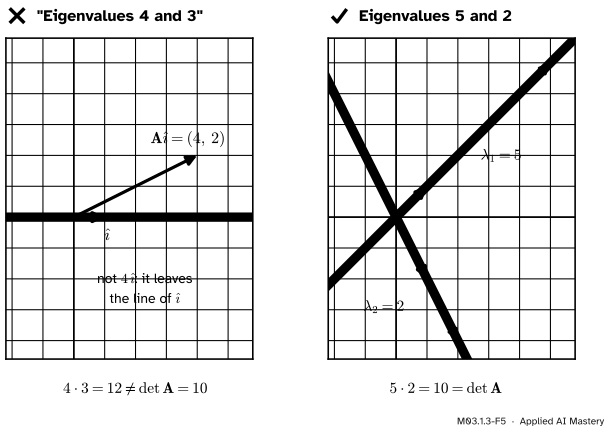
Wrong beside right. Reading the eigenvalues off the diagonal of \(\mat{A}\) gives 4 and 3. Their sum matches the trace, as the diagonal of any matrix does, but their product fails the determinant check.
“The eigenvalues are the diagonal entries.”
Only for triangular (and diagonal) matrices. For \(\mat{A}\), 4 and 3 add up to the trace, as the diagonal entries of any matrix do, but \({4 \cdot 3} = 12 \neq 10\). Always check both the sum and the product.
“The eigenvalues of a sum are the sums of the eigenvalues.”
That is safe when the two matrices share their eigenvectors, as \(\mat{A}\) and \(3\mat{I}\) do, and in general it fails. The matrices with rows \((0, 1), (0, 0)\) and \((0, 0), (1, 0)\) both have only the eigenvalue 0, yet their sum, with rows \((0, 1)\) and \((1, 0)\), has eigenvalues 1 and \(-1\). Products fail in the same way: their product, with rows \((1, 0)\) and \((0, 0)\), has eigenvalue 1.
“A repeated eigenvalue brings two independent eigenvectors.”
The shear has \(\lambda = 1\) twice and one line of eigenvectors. Count the dimension of \(E_\lambda\), never the repeats in the polynomial. This is the case where the good basis of M02.9.4 does not exist, and M03.2.1 will meet it again.
Check yourself
Recall
1. What do the eigenvalues of a square matrix add up to, and what do they multiply to?
Show answer
They add up to the trace and multiply to the determinant, counted with repeats.
2. What is the eigenspace \(E_\lambda\), and why is it a subspace?
Show answer
The null space of \(\mat{A} - \lambda\mat{I}\): every eigenvector for \(\lambda\) plus \(\vect{0}\). A null space is closed under adding and scaling, so it is a subspace.
3. Give the algebraic and geometric multiplicity of \(\lambda = 1\) for the identity and for the shear.
4. If \({\mat{A}\vect{v}} = {\lambda\vect{v}}\), what are the eigenvalues of \(\mat{A}^k\), \(\mat{A}^{-1}\) and \(\mat{A} + c\mat{I}\) for \(\vect{v}\)?
Show answer
\(\lambda^k\), \(\frac{1}{\lambda}\) (when \(\mat{A}\) is invertible) and \({\lambda + c}\).
5. Why do similar matrices have the same eigenvalues?
Show answer
\({\det(\mat{P}^{-1}\mat{A}\mat{P} - \lambda\mat{I})} = {\det(\mat{P}^{-1}(\mat{A} - \lambda\mat{I})\mat{P})}\), which equals \({\det(\mat{A} - \lambda\mat{I})}\) by the product rule, so they share the characteristic polynomial.
Exercises
1.★ A 2 by 2 matrix has trace 6 and determinant 8. Find its eigenvalues. Another has trace 10 and one eigenvalue 3: what is the other, and what is its determinant?
Show solution
The first satisfies \({\lambda^2 - 6\lambda + 8} = {(\lambda - 4)(\lambda - 2)}\), so 4 and 2. For the second, the eigenvalues add up to 10, so the other is \({10 - 3} = 7\) and the determinant is \({3 \cdot 7} = 21\).
2.★★ For the running \(\mat{A}\), find the eigenvalues of \(\mat{A}^3\) and of \(\mat{A} - 5\mat{I}\) without computing the matrices. Is \(\mat{A} - 5\mat{I}\) invertible?
Show solution
\(\mat{A}^3\) has \({5^3} = 125\) and \({2^3} = 8\). \(\mat{A} - 5\mat{I}\) has \({5 - 5} = 0\) and \({2 - 5} = -3\). Its determinant is the product, \({0 \cdot (-3)} = 0\), so it is not invertible: it crushes the line of \((1, 1)\) to the origin, as in the anchor figure of the last lesson.
3.★★★ Find the eigenvalues of \(\begin{bmatrix} 2 & 1 & 0 \\ 0 & 2 & 0 \\ 0 & 0 & 3 \end{bmatrix}\) with their algebraic and geometric multiplicities. Do its eigenvectors give a basis of \(\R^3\)?
Show solution
The matrix is triangular, so its characteristic polynomial is \({(2 - \lambda)^2(3 - \lambda)}\): \(\lambda = 2\) with algebraic multiplicity 2 and \(\lambda = 3\) with algebraic multiplicity 1.
For \(\lambda = 2\) the shifted matrix has rows \((0, 1, 0)\), \((0, 0, 0)\) and \((0, 0, 1)\). They say \(y = 0\) and \(z = 0\), with \(x\) free, so \(E_2\) is the line of \((1, 0, 0)\): geometric multiplicity 1. For \(\lambda = 3\) the rows are \((-1, 1, 0)\), \((0, -1, 0)\) and \((0, 0, 0)\), so \(y = 0\), then \(x = 0\), with \(z\) free: \(E_3\) is the line of \((0, 0, 1)\), geometric multiplicity 1.
Altogether the eigenspaces supply only two independent directions, \((1, 0, 0)\) and \((0, 0, 1)\), so there is no basis of \(\R^3\) made of eigenvectors. The top-left block is a shear in disguise.
Summary card
The eigenvalues add up to the trace and multiply to the determinant.
M03.1.3-F1
Areas grow by \(5 \times 2 = \det\mat{A}\).
Sum and product.\({\lambda_1 + \cdots + \lambda_n} = \operatorname{tr}(\mat{A})\), \({\lambda_1 \cdots \lambda_n} = \det\mat{A}\).
Eigenspace.\(E_\lambda\) is the null space of \(\mat{A} - \lambda\mat{I}\).
Multiplicities.\(1 \le\) geometric \(\le\) algebraic; the shear has 1 and 2.
Independence. Different eigenvalues give independent eigenvectors.
Related matrices.\(\lambda^k\), \(\frac{1}{\lambda}\), \({\lambda + c}\); similar matrices share \(\lambda\).
Sources and next steps
Sources. Each was opened and checked against this lesson on 15 November 2026.
Gilbert Strang, Eigenvalues and eigenvectors, MIT OpenCourseWare 18.06SC, lecture 21, and its lecture summary. The sum of the eigenvalues is the trace and their product is the determinant; adding \(3I\) adds 3 to each eigenvalue and keeps the eigenvectors; the caution that eigenvalues of sums and products are not usually sums and products; the triangular matrix with a repeated eigenvalue and only one independent eigenvector.
Dan Margalit and Joseph Rabinoff, Interactive Linear Algebra (open textbook, Georgia Tech): Section 5.1, the fact that eigenvectors with distinct eigenvalues are linearly independent; Section 5.3, similar matrices have the same characteristic polynomial, eigenvalues, trace and determinant; Section 5.4, algebraic and geometric multiplicity, the bound between them, and the shear with multiplicities 2 and 1 beside the identity with 2 and 2.
Sheldon Axler, Linear Algebra Done Right, 4th edition (open access). Result 5.11: every list of eigenvectors with distinct eigenvalues is linearly independent, proved with a shortest dependent list as in the collapsed block above.