The matrix of a linear map depends on the basis used to write it. Derive the rule that the new matrix is P inverse times A times P by translating in, acting and translating out, work it by hand for the course’s running map, and prove that the determinant does not change.
Explain what the matrix of a linear map in a basis B records: where the vectors of B land, written in the coordinates of B.
Derive the rule that the matrix of a map in a new basis is P inverse times A times P.
Compute the matrix of a map in a new basis by hand and check it on a vector.
Prove that similar matrices have the same determinant, and use the fact that they have the same trace.
In review. The maths and code on this page are checked by automated tests on every change, but an independent reader has not signed it off yet. Spot a mistake or a confusing step? Tell us.
The question
The course’s running map \(T(x, y) = {(x + y,\; -x + 2y)}\) has the matrix with columns \((1, -1)\) and \((1, 2)\). Those numbers came from watching where \(\ihat\) and \(\jhat\) land. Someone who counts on the grid of \(\vect{b}_1, \vect{b}_2\) watches different arrows and writes a different matrix for the very same map. Which matrix? And if two people write different matrices for one map, is there anything about the map that they must still agree on?
From the last lesson
1. Which way does \(\mat{P}\) translate, and which way does \(\mat{P}^{-1}\) translate?
Show answer
\(\mat{P}\) takes new coordinates to standard ones, \(\vect{v} = \mat{P}\,[\vect{v}]_B\). Its inverse takes standard coordinates to new ones, \([\vect{v}]_B = \mat{P}^{-1}\vect{v}\).
2. How do you build the change-of-basis matrix of a basis?
Show answer
Write the basis vectors, in standard coordinates, as the columns of a matrix, in the order of the basis.
Intuition
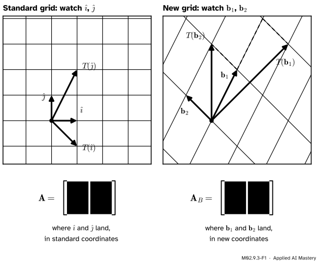
A matrix is a record of where the basis vectors land (lesson M02.4.2). That record is written in a language. The usual matrix \(\mat{A}\) of \(T\) watches \(\ihat\) and \(\jhat\), and writes down where they land in standard coordinates.
A person who works in the basis \(B\), with \(\vect{b}_1 = (1, 2)\) and \(\vect{b}_2 = (-1, 1)\), keeps the same kind of record in their own language. They watch \(\vect{b}_1\) and \(\vect{b}_2\), and they write down where those land as steps of \(\vect{b}_1\) and \(\vect{b}_2\).
M02.9.3-F1
One map, two records. \(\mat{A}\) lists where \(\ihat\) and \(\jhat\) land, in standard coordinates. \(\mat{A}_B\) lists where \(\vect{b}_1\) and \(\vect{b}_2\) land, in the coordinates of \(B\). The images in both panels come from the same map \(T\).
On the right, follow the dashed lines. \(T(\vect{b}_1)\) is two steps of \(\vect{b}_1\) and one step against \(\vect{b}_2\), so the first column of the new record is \((2, -1)\). \(T(\vect{b}_2)\) is one step of each, so the second column is \((1, 1)\). The map is the same. Only the bookkeeping differs.
Build it up
Step 1. Say what the new matrix must do. The matrix of \(T\) in the basis \(B\), written \(\mat{A}_B\), works entirely in \(B\)’s language: give it the new coordinates of an input and it returns the new coordinates of the image.
Step 2. Find its columns by watching the basis. Apply \(T\) to each basis vector, then translate the result into \(B\) with \(\mat{P}^{-1} = \tfrac13\begin{bmatrix} 1 & 1 \\ -2 & 1 \end{bmatrix}\) from the last lesson:
These are the two columns of \(\mat{A}_B\), exactly as the figure showed.
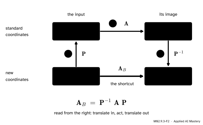
Step 3. Or take any input on a three-step trip. We already own a matrix for \(T\), but it speaks the standard language. So translate in, let it act, and translate out.
M02.9.3-F2
Three steps round the top give the same result as the shortcut along the bottom. 1\(\mat{P}\) translates the input into standard coordinates. 2\(\mat{A}\) acts. 3\(\mat{P}^{-1}\) translates the image back.
Step 4. Three matrices in a row are one matrix. Doing one map after another multiplies their matrices, with the first map on the right (module M02.5). So the whole trip is the single matrix \(\mat{P}^{-1}\mat{A}\mat{P}\), and that is \(\mat{A}_B\).
The formal statement
NoteDefinition and result: the matrix of a map in a basis
Let \(T\) be a linear map from \(\R^n\) to itself and let \(B\) be a basis of \(\R^n\). The matrix of \(T\) in the basis \(B\) is the matrix \(\mat{A}_B\) for which
The first holds because the inverse of \(\mat{P}\) translates into \(B\). The second holds because \(\mat{A}\) is the standard matrix of \(T\), so \(T(\vect{x}) = \mat{A}\vect{x}\). The third puts \(\vect{x} = \mat{P}\,[\vect{x}]_B\).
So \(\mat{P}^{-1}\mat{A}\mat{P}\) turns \([\vect{x}]_B\) into \([T(\vect{x})]_B\) for every \(\vect{x}\). Every list of \(n\) numbers \(\vect{c}\) is the coordinate vector of some \(\vect{x}\), namely \(\vect{x} = \mat{P}\vect{c}\). So we know what the matrix does to every input, and a linear map has only one matrix (lesson M02.4.2). Hence \(\mat{A}_B = \mat{P}^{-1}\mat{A}\mat{P}\). \(\blacksquare\)
The two outer matrices change the point of view. The middle one is the map as the standard basis sees it.
Two matrices related in this way are called similar: \(\mat{M}\) is similar to \(\mat{A}\) when \(\mat{M} = \mat{P}^{-1}\mat{A}\mat{P}\) for some invertible \(\mat{P}\). Similar matrices are the same map described in different bases.
What cannot change: the determinant. Module M02.8 showed that the determinant of a product is the product of the determinants, and that \(\det(\mat{P}^{-1}) = 1/\det(\mat{P})\). Therefore
This had to be true. The determinant is the factor by which the map scales areas, and that is a fact about the map, not about the grid used to describe it.
What cannot change: the trace. The trace of a square matrix, \(\operatorname{tr}(\mat{A})\), is the sum of the entries on its diagonal. Similar matrices also have the same trace: \(\operatorname{tr}(\mat{P}^{-1}\mat{A}\mat{P}) = \operatorname{tr}(\mat{A})\).
Go deeper: why the trace survives a change of basis
The key fact is that \(\operatorname{tr}(\mat{X}\mat{Y}) = \operatorname{tr}(\mat{Y}\mat{X})\) for square matrices of the same size, even though \(\mat{X}\mat{Y}\) and \(\mat{Y}\mat{X}\) usually differ. The entry in row \(i\), column \(i\) of \(\mat{X}\mat{Y}\) is \(\sum_k x_{ik}\,y_{ki}\), so
The middle step only swaps the order of adding and the order of each product of two numbers. Now take \(\mat{X} = \mat{P}^{-1}\) and \(\mat{Y} = \mat{A}\mat{P}\):
The first step is the key fact. The second uses the fact that matrix multiplication is associative (lesson M02.5.3). The third uses \(\mat{P}\mat{P}^{-1} = \mat{I}\).
Worked example
Find the matrix of \(T(x, y) = {(x + y,\; -x + 2y)}\) in the basis \(\vect{b}_1 = (1, 2)\), \(\vect{b}_2 = (-1, 1)\), and test it on \(\vect{x} = (2, 1)\).
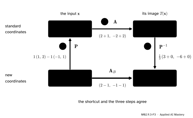
Test it. From lesson M02.9.1, \(\vect{x} = (2, 1)\) has \([\vect{x}]_B = (1, -1)\).
M02.9.3-F3
The input \(\vect{x} = (2, 1)\) followed both ways. Three steps round the top and one step along the bottom reach the same new coordinates, \((1, -2)\).
The three steps: \(\mat{P}\,(1, -1) = (2, 1)\). Then \(\mat{A}\,(2, 1) = (3, 0)\). Then \(\mat{P}^{-1}(3, 0) = \tfrac13\,(3, -6) = (1, -2)\). They agree. As a last check, \((1, -2)\) in \(B\) is the arrow \(1\,(1, 2) - 2\,(-1, 1) = (3, 0)\), which is \(T(2, 1)\).
What the two records agree on.\(\det(\mat{A}) = {1 \cdot 2} - {1 \cdot (-1)} = 3\) and \(\det(\mat{A}_B) = {2 \cdot 1} - {1 \cdot (-1)} = 3\). \(\operatorname{tr}(\mat{A}) = 1 + 2 = 3\) and \(\operatorname{tr}(\mat{A}_B) = 2 + 1 = 3\).
Code
From scratch, with exact fractions so that no rounding hides a mistake.
from fractions import Fractiondef matmul(X, Y):"""The product of two 2 by 2 matrices, each a list of rows."""return [[sum(X[i][k] * Y[k][j] for k inrange(2)) for j inrange(2)]for i inrange(2)]def inverse(M): (p, q), (r, s) = M cell = Fraction(p * s - q * r)return [[s / cell, -q / cell], [-r / cell, p / cell]]A = [[1, 1], [-1, 2]] # the running map T, in the standard basisP = [[1, -1], [2, 1]] # columns are b1 and b2AP = matmul(A, P)A_B = matmul(inverse(P), AP)show =lambda M: [[str(entry) for entry in row] for row in M]print("A P =", show(AP))print("P^-1 A P =", show(A_B))print("wrong order =", show(matmul(matmul(P, A), inverse(P))))
A P          = [['3', '0'], ['3', '3']]
P^-1 A P     = [['2', '1'], ['-1', '1']]
wrong order  = [['4/3', '1/3'], ['-7/3', '5/3']]
Now NumPy, with the checks that the lesson made by hand.
import numpy as npA = np.array([[1.0, 1.0], [-1.0, 2.0]])P = np.array([[1.0, -1.0], [2.0, 1.0]])A_B = np.linalg.solve(P, A @ P) # P^-1 (A P), with no inverse formedx = np.array([2.0, 1.0])x_B = np.linalg.solve(P, x)print("A_B =\n", A_B)print("shortcut: ", A_B @ x_B)print("three steps:", np.linalg.solve(P, A @ (P @ x_B)))print("determinants:", np.linalg.det(A).round(6), np.linalg.det(A_B).round(6))print("traces: ", np.trace(A), np.trace(A_B))
The hidden cell at the end repeats the determinant and trace checks on two hundred random 3 by 3 maps and bases. The rule is not special to the plane.
Explore
This module’s interactive, the two-grid viewer, lives in lesson M02.9.2. Set the arrow to \((2, 1)\) and then to \((3, 0)\) there, with the module basis. The new coordinates it reports, \((1, -1)\) and \((1, -2)\), are the input and output of \(\mat{A}_B\) in the worked example.
Pitfalls
M02.9.3-F4
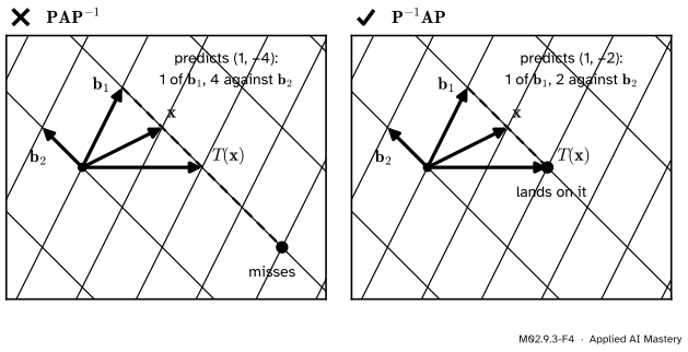
Wrong beside right. With the three matrices in the wrong order, the predicted image of \(\vect{x}\) misses the true one. In the right order it lands on it.
“\(\mat{P}\mat{A}\mat{P}^{-1}\) or \(\mat{P}^{-1}\mat{A}\mat{P}\): the order cannot matter much.”
It matters completely. Here \(\mat{P}\mat{A}\mat{P}^{-1} = \tfrac13\begin{bmatrix} 4 & 1 \\ -7 & 5 \end{bmatrix}\). Applied to \([\vect{x}]_B = (1, -1)\) it gives \((1, -4)\), which names the arrow \((5, -2)\) and not \(T(\vect{x}) = (3, 0)\). To get the order right, read from the right and ask what each matrix accepts. The input is in new coordinates, so the first matrix to act must be \(\mat{P}\).
“The entries changed, so it is a different map.”
\(\mat{A}\) and \(\mat{A}_B\) share no column, yet they are one map. Be careful, then, about reading meaning into single entries of a matrix. In machine learning, the entries of a matrix that maps a space to itself depend on the basis chosen for that space. Its determinant and its trace do not, and neither do the eigenvalues that course M03 introduces. Those are the numbers that describe the map itself.
“Same determinant and same trace, so the matrices are similar.”
The rule runs one way only. The identity \(\begin{bmatrix} 1 & 0 \\ 0 & 1 \end{bmatrix}\) and the shear \(\begin{bmatrix} 1 & 1 \\ 0 & 1 \end{bmatrix}\) both have determinant 1 and trace 2. But \(\mat{P}^{-1}\mat{I}\mat{P} = \mat{P}^{-1}\mat{P} = \mat{I}\) for every \(\mat{P}\), so the identity is similar only to itself. Doing nothing looks like doing nothing in every basis.
Check yourself
Recall
1. What does the matrix \(\mat{A}_B\) take in, and what does it give out?
Show answer
It takes the coordinates of an input in the basis \(B\) and gives the coordinates of its image in the basis \(B\): \(\mat{A}_B\,[\vect{x}]_B = [T(\vect{x})]_B\).
2. State the rule for \(\mat{A}_B\) and say what each of the three matrices does.
Show answer
\(\mat{A}_B = \mat{P}^{-1}\mat{A}\mat{P}\). Reading from the right: \(\mat{P}\) translates the input into standard coordinates, \(\mat{A}\) applies the map, and \(\mat{P}^{-1}\) translates the image back.
3. What do the columns of \(\mat{A}_B\) hold?
Show answer
Where the basis vectors of \(B\) land, written in the coordinates of \(B\): column \(j\) is \([T(\vect{b}_j)]_B\).
4. What does it mean for two matrices to be similar?
Show answer
One is \(\mat{P}^{-1}\) times the other times \(\mat{P}\) for some invertible \(\mat{P}\). They describe the same linear map in two different bases.
5. Name two numbers that similar matrices always share.
Show answer
The determinant and the trace.
Exercises
1.★ The vector \(\vect{v} = (1, 5)\) has \([\vect{v}]_B = (2, 1)\). Use \(\mat{A}_B = \begin{bmatrix} 2 & 1 \\ -1 & 1 \end{bmatrix}\) to find \([T(\vect{v})]_B\), and check it against \(T(1, 5)\) computed directly.
Directly, \(T(1, 5) = {(1 + 5,\; -1 + 10)} = (6, 9)\). And \((5, -1)\) in \(B\) is the arrow \(5\,(1, 2) - 1\,(-1, 1) = {(5 + 1,\; 10 - 1)} = (6, 9)\). They agree.
2.★★ Find the matrix of the shear \(\mat{H} = \begin{bmatrix} 1 & 1 \\ 0 & 1 \end{bmatrix}\) in the basis \((1, 1), (0, 1)\). Confirm that the determinant and the trace are unchanged.
Show solution
\(\mat{P} = \begin{bmatrix} 1 & 0 \\ 1 & 1 \end{bmatrix}\) has \({ps - qr} = 1\), so \(\mat{P}^{-1} = \begin{bmatrix} 1 & 0 \\ -1 & 1 \end{bmatrix}\). Then
Determinant: \({2 \cdot 0} - {1 \cdot (-1)} = 1\), the same as \({1 \cdot 1} - {1 \cdot 0} = 1\). Trace: \(2 + 0 = 2\), the same as \(1 + 1 = 2\).
A check by columns: \(\mat{H}\,(1, 1) = (2, 1) = 2\,(1, 1) - 1\,(0, 1)\), which is the first column \((2, -1)\).
3.★★★ Let \(\mat{M} = \mat{P}^{-1}\mat{A}\mat{P}\). Show that \(\mat{M}^2 = \mat{P}^{-1}\mat{A}^2\mat{P}\), and then that \(\mat{M}^k = \mat{P}^{-1}\mat{A}^k\mat{P}\) for every whole number \(k \ge 1\).
Show solution
Write out the square and regroup, which is allowed because matrix multiplication is associative:
It holds for \(k = 1\) by definition, so it holds for \(k = 2\), then \(k = 3\), and so on for every \(k\). In words: repeating a map \(k\) times and then changing basis is the same as changing basis and then repeating. The next lesson uses this to compute powers quickly.
Summary card
Translate in, act, translate out: \(\mat{A}_B = \mat{P}^{-1}\mat{A}\mat{P}\).
M02.9.3-F1
One map, two records.
Meaning.\(\mat{A}_B\,[\vect{x}]_B = [T(\vect{x})]_B\), and column \(j\) of \(\mat{A}_B\) is \([T(\vect{b}_j)]_B\).
The rule.\(\mat{A}_B = \mat{P}^{-1}\mat{A}\mat{P}\), read from the right.
Similar matrices are one map in two bases.
Unchanged.\(\det(\mat{P}^{-1}\mat{A}\mat{P}) = \det(\mat{A})\) and \(\operatorname{tr}(\mat{P}^{-1}\mat{A}\mat{P}) = \operatorname{tr}(\mat{A})\).
Sources and next steps
Sources. Each was opened and checked against this lesson on 12 November 2026.
Sheldon Axler, Linear Algebra Done Right, 4th edition (open access). Result 3.84 is the change-of-basis formula, \(A = C^{-1}BC\). Definition 8.47 is the trace, result 8.49 is \(\operatorname{tr}(AB) = \operatorname{tr}(BA)\), and result 8.50 uses it to show that the trace of the matrix of an operator does not depend on the basis.
Dan Margalit and Joseph Rabinoff, Interactive Linear Algebra, Section 5.3, Similarity (open textbook, Georgia Tech). It defines similar matrices, explains that they do the same thing in different coordinate systems, and notes that they share trace and determinant. It also gives the shear and the identity as two matrices that are not similar although they have the same characteristic polynomial, and therefore the same trace and determinant.
Grant Sanderson, Change of basis, 3Blue1Brown, Linear Algebra, chapter 13. The source of the reading of \(A^{-1}MA\) used here: the middle matrix is the transformation as we see it and the outer two are the shift in perspective.
Gilbert Strang, Change of basis; image compression, MIT OpenCourseWare 18.06SC, lecture 31. The lecture summary states that the matrices of one transformation in two bases are similar, \(B = M^{-1}AM\).
Next.M02.9.4 Choosing a good basis asks which basis makes \(\mat{P}^{-1}\mat{A}\mat{P}\) as simple as a matrix can be.