When does a product of two matrices exist, and what shape is it? Meet the shape rule, the identity matrix and powers of a matrix, then see a stack of neural-network layers collapse into one matrix, and why a non-linearity between the layers stops that.
Decide from the shapes of two matrices whether their product exists, and state the shape of the result.
Explain why multiplying by the identity matrix changes nothing, and which size of identity fits on each side.
Compute powers of a square matrix and read them as one map applied again and again.
Write a stack of linear layers as a single product of matrices, and explain why a network needs a non-linearity between its layers.
In review. The maths and code on this page are checked by automated tests on every change, but an independent reader has not signed it off yet. Spot a mistake or a confusing step? Tell us.
The question
One layer of a network turns the 784 pixels of a small image into 128 numbers. The next layer turns those 128 into 10 scores. Each layer is a matrix, so the two together are a product of matrices. Which products are allowed at all? And if a hundred layers multiply out to one matrix, why does anyone build a deep network?
From the last lesson
1. Is \(\mat{A}\mat{B} = \mat{B}\mat{A}\) for all matrices? Give an example.
Show answer
No. For the shear \(\mat{S}\) and the quarter turn \(\mat{R}\), \(\mat{R}\mat{S} = \begin{bmatrix} 0 & -1 \\ 1 & 1 \end{bmatrix}\) and \(\mat{S}\mat{R} = \begin{bmatrix} 1 & -1 \\ 1 & 0 \end{bmatrix}\).
2. State the associative law, and say what it means for maps.
Show answer
\((\mat{A}\mat{B})\mat{C} = \mat{A}(\mat{B}\mat{C})\). Either way a vector meets \(\mat{C}\), then \(\mat{B}\), then \(\mat{A}\). The brackets only say which pair was merged first.
Intuition
A product \(\mat{A}\mat{B}\) means “first \(\mat{B}\), then \(\mat{A}\)”. For that to make sense, what comes out of \(\mat{B}\) must be something that \(\mat{A}\) can take in. Think of plumbing: two pipes join only if the ends that meet are the same size.
M02.4.4 read the shape of a matrix as “outputs by inputs”: an \(m \times n\) matrix takes \(n\) numbers in and gives \(m\) out. Write the two shapes side by side and look at the middle.
M02.5.4-F1
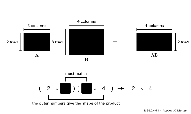
The shape rule. The number of columns of \(\mat{A}\) must equal the number of rows of \(\mat{B}\). The product has as many rows as \(\mat{A}\) and as many columns as \(\mat{B}\).
In the figure, \(\mat{B}\) takes 4 numbers in and gives 3 out. \(\mat{A}\) takes those 3 in and gives 2 out. The journey takes 4 numbers to 2, so the product is \(2 \times 4\).
Build it up
Step 1. The shape rule. Let \(\mat{B}\) be \(n \times p\): it takes \(p\) numbers in and gives \(n\) out. Let \(\mat{A}\) be \(m \times n\): it takes \(n\) in and gives \(m\) out. The two \(n\)’s are the join. The product \(\mat{A}\mat{B}\) takes \(p\) numbers in and gives \(m\) out, so it is \(m \times p\).
For \(\mat{A}\mat{B}\) the shapes read \((2 \times 3)(3 \times 2)\): the middle numbers are 3 and 3, so the product exists and is \(2 \times 2\). For \(\mat{B}\mat{A}\) they read \((3 \times 2)(2 \times 3)\): the middle numbers are 2 and 2, so this product exists too, and it is \(3 \times 3\). The two orders do not even have the same shape. And \(\mat{A}\mat{A}\) would read \((2 \times 3)(2 \times 3)\), with 3 and 2 in the middle: it does not exist.
Step 3. The matrix that does nothing. The identity matrix\(\mat{I}\) has ones down its diagonal and zeros elsewhere. Its columns are the basis vectors themselves, so it sends every vector to itself. Doing nothing before or after a map changes nothing: \(\mat{A}\mat{I} = \mat{A}\) and \(\mat{I}\mat{A} = \mat{A}\). It plays the part of the number 1.
Step 4. The same map, again and again. If a matrix is square, its outputs fit its own inputs, so it can be multiplied by itself. \(\mat{A}^2 = \mat{A}\mat{A}\) means “apply \(\mat{A}\) twice”, and \(\mat{A}^k\) means “apply it \(k\) times”.
M02.5.4-F2
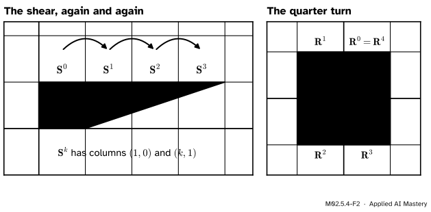
Two families of powers. Each extra shear slides the top of the square one more unit. Each extra quarter turn moves the square to the next quarter of the plane, and the fourth brings it home.
For the shear, \(\mat{S}^k = \begin{bmatrix} 1 & k \\ 0 & 1 \end{bmatrix}\). For the quarter turn, two turns make a half turn, \(\mat{R}^2 = \begin{bmatrix} -1 & 0 \\ 0 & -1 \end{bmatrix}\), and four make a full turn, \(\mat{R}^4 = \mat{I}\).
Step 5. A stack of layers is a product. Ignore biases for a moment. A layer multiplies its input by a weight matrix (M02.4.4). Feed the output of layer 1 into layer 2:
Two layers have become one matrix. For the network in the opening question, \(\mat{W}_1\) is \(128 \times 784\) and \(\mat{W}_2\) is \(10 \times 128\). The shapes read \((10 \times 128)(128 \times 784)\), so the product is \(10 \times 784\). The two layers hold \(100{,}352 + 1{,}280 = 101{,}632\) weights, and together they do exactly what a single matrix with \(7{,}840\) entries does. Something must be added to make depth worth having.
The formal statement
NoteResult 1: the shape rule
If \(\mat{A}\) is \(m \times n\) and \(\mat{B}\) is \(n \times p\), then \(\mat{A}\mat{B}\) exists and is \(m \times p\). If the number of columns of \(\mat{A}\) differs from the number of rows of \(\mat{B}\), the product is not defined.
Why. Column \(j\) of \(\mat{A}\mat{B}\) is \(\mat{A}\vect{b}_j\) (M02.5.2). The column \(\vect{b}_j\) has as many entries as \(\mat{B}\) has rows, and \(\mat{A}\vect{b}_j\) is defined only when that number equals the number of columns of \(\mat{A}\) (M02.4.4). When it is, \(\mat{B}\) has \(p\) columns, so the product has \(p\) columns, and each \(\mat{A}\vect{b}_j\) has \(m\) entries, so it has \(m\) rows.
NoteDefinition and Result 2: the identity matrix
The \(n \times n\)identity matrix\(\mat{I}_n\) has columns \(\vect{e}_1, \dots, \vect{e}_n\). For every \(m \times n\) matrix \(\mat{A}\),
Proof. First, \(\mat{I}_n\vect{x} = x_1\vect{e}_1 + \cdots + x_n\vect{e}_n = \vect{x}\) for every \(\vect{x}\), by the column view. Now compare columns. Column \(j\) of \(\mat{A}\mat{I}_n\) is \(\mat{A}\vect{e}_j\), which is column \(j\) of \(\mat{A}\) (M02.4.2). Column \(j\) of \(\mat{I}_m\mat{A}\) is \(\mat{I}_m\vect{a}_j = \vect{a}_j\). In both cases every column is the matching column of \(\mat{A}\).
For a \(2 \times 3\) matrix, \(\mat{I}_3\) fits on the right and \(\mat{I}_2\) on the left.
NoteDefinition: powers
For a square matrix \(\mat{A}\) and a whole number \(k \geq 1\), \(\mat{A}^k\) is the product of \(k\) copies of \(\mat{A}\). By convention \(\mat{A}^0 = \mat{I}\): applying a map no times moves nothing.
No brackets are needed, because multiplication is associative (M02.5.3). For the same reason \(\mat{A}^j\mat{A}^k = \mat{A}^{j+k}\): the left side is \(j\) copies followed by \(k\) copies, which is \(j + k\) copies in a row.
The powers of the shear. Suppose \(\mat{S}^k = \begin{bmatrix} 1 & k \\ 0 & 1 \end{bmatrix}\) for some \(k\). One more factor gives
The formula is true for \(k = 1\), and each step carries it from \(k\) to \(k + 1\), so it is true for every \(k\).
One caution: \((\mat{A}\mat{B})^2\) is \(\mat{A}\mat{B}\mat{A}\mat{B}\), not \(\mat{A}^2\mat{B}^2 = \mat{A}\mat{A}\mat{B}\mat{B}\). The two agree when \(\mat{A}\) and \(\mat{B}\) commute, since the middle pair can then be swapped. Otherwise they usually differ: for the quarter turn and the shear, \((\mat{R}\mat{S})^2 = \begin{bmatrix} -1 & -1 \\ 1 & 0 \end{bmatrix}\) but \(\mat{R}^2\mat{S}^2 = \begin{bmatrix} -1 & -2 \\ 0 & -1 \end{bmatrix}\).
NoteResult 3: linear layers collapse
For weight matrices \(\mat{W}_1, \mat{W}_2, \dots, \mat{W}_L\) whose shapes fit,
A stack of linear layers, however deep, computes what one matrix computes.
Why. For two layers this is \(\mat{A}(\mat{B}\vect{x}) = (\mat{A}\mat{B})\vect{x}\) from M02.5.2. Each further layer repeats the argument, with the product so far in the place of \(\mat{B}\). Biases do not rescue depth. Multiplying by \(\mat{W}_2\) is additive, so (Exercise 3 of M02.5.1)
What stops the collapse. Put a function that is not linear between the layers. The most common choice is the ReLU, \(\operatorname{relu}(z) = \max(z, 0)\), applied to every entry of a vector. It fails additivity: \(\operatorname{relu}(1) + \operatorname{relu}(-1) = 1 + 0 = 1\), but \(\operatorname{relu}(1 + (-1)) = \operatorname{relu}(0) = 0\). So \(\vect{x} \mapsto \mat{W}_2\operatorname{relu}(\mat{W}_1\vect{x})\) is no longer forced to be a linear map.
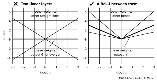
A network with one input shows this. Let \(\mat{W}_1 = \begin{bmatrix} 1 \\ -1 \end{bmatrix}\) and \(\mat{W}_2 = \begin{bmatrix} 1 & 1 \end{bmatrix}\). The hidden layer is \((x, -x)\). With the ReLU the output is \(\max(x, 0) + \max(-x, 0) = \abs{x}\). Without it the output is \(x + (-x) = 0\) for every input, as it must be, since \(\mat{W}_2\mat{W}_1 = \begin{bmatrix} 1 \cdot 1 + 1 \cdot (-1) \end{bmatrix} = \begin{bmatrix} 0 \end{bmatrix}\). And \(\abs{x}\) is beyond any matrix: \(\abs{1} + \abs{-1} = 2\), but \(\abs{1 + (-1)} = 0\).
Go deeper: why the product in the worked example has two equal rows
The worked example below gets \(\begin{bmatrix} 1 & 2 \\ 1 & 2 \end{bmatrix}\), with equal rows. The first matrix places the plane in space as the sheet of points \((x, y, x + y)\). The second squashes space along \((2, -1, 1)\) (M02.4.4), a direction that lies in that sheet, because \(2 + (-1) = 1\). So the sheet lands on a line: every output is \((x + 2y,\; x + 2y)\). M02.7 takes this up with the idea of rank.
Frontier note: powers of a matrix inside a recurrent network
A recurrent network applies the same weights at every time step, so its gradient over many steps contains a long product of matrices. With no non-linearity, that product is a power of one matrix, and powers grow or shrink fast: scaling the plane by \(1.1\), fifty times over, scales it by \(1.1^{50} \approx 117\), and with \(0.9\) the factor is about \(0.005\). Pascanu, Mikolov and Bengio (2013) trace the exploding and vanishing gradient problems to this. The factors in the gradient, they write, “take the form of a product of \(t - k\) Jacobian matrices. In the same way a product of \(t - k\) real numbers can shrink to zero or explode to infinity, so does this product of matrices”. With no non-linearity, the paper gives the condition in terms of the eigenvalues of the weight matrix (M03.1): the long-term part of the gradient vanishes if the largest is smaller than 1 in absolute value, and the gradient can explode only if it is larger than 1 in absolute value.
Worked example
A network has two linear layers and no non-linearity: 2 inputs, 3 hidden units, 2 outputs. Its weights are the matrices of Step 2, \(\mat{W}_1 = \mat{B}\) and \(\mat{W}_2 = \mat{A}\). Find the single matrix that does the same job.
M02.5.4-F3
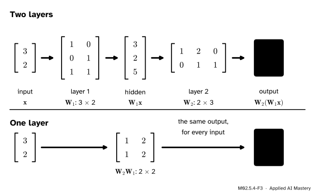
The input \((3, 2)\) sent through the two layers one after the other, and through the single product matrix. Both give \((7, 7)\).
Check the shapes. The job is “first \(\mat{W}_1\), then \(\mat{W}_2\)”, so the matrix is \(\mat{W}_2\mat{W}_1\). The shapes read \((2 \times 3)(3 \times 2)\): the middle numbers match, and the product is \(2 \times 2\).
Multiply, row times column. The rows of \(\mat{W}_2\) are \((1, 2, 0)\) and \((0, 1, 1)\). The columns of \(\mat{W}_1\) are \((1, 0, 1)\) and \((0, 1, 1)\).
def shape(A):return (len(A), len(A[0]))def matmul(A, B):"""A times B. The number of columns of A must equal the number of rows of B.""" (m, n), (rows_b, p) = shape(A), shape(B)if n != rows_b:raiseValueError(f"({m} x {n})({rows_b} x {p}): the middle numbers {n} and {rows_b} differ")return [[sum(A[i][k] * B[k][j] for k inrange(n)) for j inrange(p)] for i inrange(m)]A = [[1, 2, 0], [0, 1, 1]] # 2 by 3B = [[1, 0], [0, 1], [1, 1]] # 3 by 2print("A B =", matmul(A, B), " shape", shape(matmul(A, B)))print("B A =", matmul(B, A), " shape", shape(matmul(B, A)))try: matmul(A, A)exceptValueErroras error:print("A A fails:", error)
A B = [[1, 2], [1, 2]]  shape (2, 2)
B A = [[1, 2, 0], [0, 1, 1], [1, 3, 1]]  shape (3, 3)
A A fails: (2 x 3)(2 x 3): the middle numbers 3 and 2 differ
The identity and powers need only a loop around matmul.
def identity(n):return [[1if i == j else0for j inrange(n)] for i inrange(n)]def power(A, k):"""A multiplied by itself k times. No times at all is the identity.""" result = identity(len(A))for _ inrange(k): result = matmul(result, A)return resultS, R, T = [[1, 1], [0, 1]], [[0, -1], [1, 0]], [[1, 1], [-1, 2]]print("A I =", matmul(A, identity(3)), " I A =", matmul(identity(2), A))print("S^5 =", power(S, 5), " R^2 =", power(R, 2), " R^4 =", power(R, 4))print("T^2 =", power(T, 2), " T^3 =", power(T, 3))
two layers: [7 7]   one matrix: [7 7]   W2 @ W1 = [[1, 2], [1, 2]]
T cubed: [[-3, 6], [-6, 3]]
x =  3:  with ReLU [3]   without [0]
x = -2:  with ReLU [2]   without [0]
V2 @ V1 = [[0]]
Last, the opening question’s network, with random weights.
rng = np.random.default_rng(0)first, second = rng.normal(size=(128, 784)), rng.normal(size=(10, 128))image = rng.normal(size=784)one = second @ firstprint("shapes:", second.shape, first.shape, "-> product", one.shape)print("weights in the two layers:", first.size + second.size, " in the one matrix:", one.size)print("same scores:", np.allclose(second @ (first @ image), one @ image))
shapes: (10, 128) (128, 784) -> product (10, 784)
weights in the two layers: 101632   in the one matrix: 7840
same scores: True
Explore
The composition explorer of this module is in lesson M02.5.3. Press Same shear twice and step through: the product in the read-out is \(\mat{S}^2\). Then use the sliders to make \(\mat{A}\) the identity, with columns \((1, 0)\) and \((0, 1)\). The second step now moves nothing, and both products equal \(\mat{B}\).
Pitfalls
M02.5.4-F4
Wrong beside right, for a network with one input, two hidden units and one output. With nothing between the layers, every choice of weights gives a straight line through the origin. With a ReLU between them, the line can bend.
“More linear layers make a more powerful model.”
They make a longer product, and a product of matrices is a matrix. Whatever the stack computes, one layer could compute. Leave the non-linearity out by mistake and the model trains without complaint, as a linear model with a great many spare weights.
“If \(\mat{A}\mat{B}\) exists, then so does \(\mat{B}\mat{A}\), with the same shape.”
A \((2 \times 3)(3 \times 4)\) product exists. In the other order the shapes read \((3 \times 4)(2 \times 3)\), with 4 and 2 in the middle: no product. Even when both exist they can differ in shape, as \(2 \times 2\) and \(3 \times 3\) did above. In NumPy a product whose middle numbers differ raises a ValueError.
“A ** 2 is the matrix \(\mat{A}\) squared.”
In NumPy, ** acts on each entry separately, like *. For \(\mat{T}\) it gives \(\begin{bmatrix} 1 & 1 \\ 1 & 4 \end{bmatrix}\). The map applied twice is T @ T, or np.linalg.matrix_power(T, 2), which is \(\begin{bmatrix} 0 & 3 \\ -3 & 3 \end{bmatrix}\).
Check yourself
Recall
1.\(\mat{A}\) is \(m \times n\) and \(\mat{B}\) is \(n \times p\). What is the shape of \(\mat{A}\mat{B}\)?
Show answer
\(m \times p\): as many rows as \(\mat{A}\) and as many columns as \(\mat{B}\).
2. When is a product \(\mat{A}\mat{B}\) not defined?
Show answer
When the number of columns of \(\mat{A}\) differs from the number of rows of \(\mat{B}\): the outputs of \(\mat{B}\) are then not valid inputs for \(\mat{A}\).
3. What are the columns of the identity matrix, and what does multiplying by it do?
Show answer
Its columns are the basis vectors \(\vect{e}_1, \dots, \vect{e}_n\). Multiplying by it changes nothing: \(\mat{A}\mat{I} = \mat{A}\) and \(\mat{I}\mat{A} = \mat{A}\).
4. What does \(\mat{A}^3\) mean as a map, and what is \(\mat{A}^0\)?
Show answer
Apply the map of \(\mat{A}\) three times. \(\mat{A}^0\) is the identity matrix: apply it no times.
5. Why does a stack of linear layers need a non-linearity between the layers?
Show answer
Without one the stack is a product of matrices, which is a single matrix: one layer could do the same.
Exercises
1.★\(\mat{A}\) is \(3 \times 4\), \(\mat{B}\) is \(4 \times 2\) and \(\mat{C}\) is \(2 \times 3\). Which of these exist, and what are their shapes? \(\mat{A}\mat{B}\), \(\mat{B}\mat{A}\), \(\mat{B}\mat{C}\), \(\mat{C}\mat{A}\), \(\mat{A}\mat{B}\mat{C}\), \(\mat{A}^2\).
\(\mat{A}\mat{B}\mat{C}\): \(\mat{A}\mat{B}\) is \(3 \times 2\), and \((3 \times 2)(2 \times 3)\) exists. The result is \(3 \times 3\).
\(\mat{A}^2\): \((3 \times 4)(3 \times 4)\), middle numbers 4 and 3. Does not exist. Only a square matrix has powers.
2.★★ (a) Let \(\mat{N} = \begin{bmatrix} 0 & 1 \\ 0 & 0 \end{bmatrix}\). Compute \(\mat{N}^2\) and explain the answer by following the basis vectors. (b) Let \(\mat{F} = \begin{bmatrix} -1 & 0 \\ 0 & 1 \end{bmatrix}\), the reflection in the vertical axis. Compute \(\mat{F}^2\). (c) Find \(\mat{R}^{2026}\) for the quarter turn \(\mat{R}\).
Show solution
(a) \(\mat{N}\) sends \(\ihat\) to \((0, 0)\) and \(\jhat\) to \((1, 0)\). Apply it twice: \(\ihat \to (0, 0) \to (0, 0)\), and \(\jhat \to (1, 0) = \ihat \to (0, 0)\). Both basis vectors end at the origin, so \(\mat{N}^2 = \begin{bmatrix} 0 & 0 \\ 0 & 0 \end{bmatrix}\). A matrix that is not zero can have a square that is.
3.★★★ Let \(f(\vect{x}) = \mat{W}_2\operatorname{relu}(\mat{W}_1\vect{x})\) be a two-layer network with a ReLU and no biases. Show that \(f(c\,\vect{x}) = c\,f(\vect{x})\) for every number \(c \geq 0\). Then use the network that computes \(\abs{x}\) to show that this fails for negative \(c\), and that \(f\) is not additive.
Show solution
First, for a single number \(z\) and \(c \geq 0\): \(\operatorname{relu}(cz) = \max(cz, 0) = c\max(z, 0) = c\operatorname{relu}(z)\), because multiplying two numbers by a non-negative \(c\) does not change which of them is larger. The same holds entry by entry for a vector. Then
The second and fourth steps use the homogeneity of \(\mat{W}_1\) and \(\mat{W}_2\), the third the fact about the ReLU.
For \(f(x) = \abs{x}\) and \(c = -1\): \(f(-1 \cdot 1) = 1\), but \(-1 \cdot f(1) = -1\). And \(f(1) + f(-1) = 2\), but \(f(1 + (-1)) = f(0) = 0\). So the network keeps homogeneity for non-negative scalings only, and loses additivity. That is the bend in the figure.
Summary card
A product exists when the middle numbers of the two shapes match.
M02.5.4-F1
Inner numbers match, outer numbers remain.
Shape rule.\((m \times n)(n \times p)\) gives \(m \times p\). Otherwise there is no product.
Identity.\(\mat{A}\,\mat{I}_n = \mat{A} = \mat{I}_m\,\mat{A}\) for an \(m \times n\) matrix \(\mat{A}\).
Powers.\(\mat{A}^k\) applies a square \(\mat{A}\)\(k\) times. \(\mat{A}^0 = \mat{I}\) and \(\mat{A}^j\mat{A}^k = \mat{A}^{j+k}\).
Layers.\(\mat{W}_2(\mat{W}_1\vect{x}) = (\mat{W}_2\mat{W}_1)\vect{x}\): linear layers collapse into one matrix.
Depth needs a bend. With \(\operatorname{relu}(z) = \max(z, 0)\) between the layers, the stack no longer has to be a single matrix.
In code.A @ B checks the shapes. np.linalg.matrix_power(A, k) is a power. A ** k is not.
Sources and next steps
Sources. Each was opened and checked against this lesson on 12 November 2026.
Sheldon Axler, Linear Algebra Done Right, 4th edition (open access). Definition 3.41 (Section 3C): an \(m\)-by-\(n\) matrix times an \(n\)-by-\(p\) matrix is \(m\)-by-\(p\), and is defined only when the first has as many columns as the second has rows. Definition 3.79 (Section 3D): the identity matrix. Notation 5.13 (Section 5A): \(T^m\), \(T^0 = I\) and \(T^mT^n = T^{m+n}\).
Marc Deisenroth, Aldo Faisal and Cheng Soon Ong, Mathematics for Machine Learning, Cambridge University Press, 2020 (free PDF). Section 2.2.1: matrices can be multiplied only if their neighbouring dimensions match (2.14); Example 2.3 multiplies a \(2 \times 3\) and a \(3 \times 2\) matrix in both orders, with \(2 \times 2\) and \(3 \times 3\) results; equation (2.20) is \(\mat{I}_m\mat{A} = \mat{A}\mat{I}_n = \mat{A}\).
Aston Zhang, Zachary Lipton, Mu Li and Alexander Smola, Dive into Deep Learning, Section 5.1. Section 5.1.1.3: a hidden layer with no activation function gains nothing, since “An affine function of an affine function is itself an affine function.” Equation (5.1.2) is the collapse with biases, and equation (5.1.4) defines the ReLU as \(\max(x, 0)\).
NumPy manual, numpy.matmul and numpy.linalg.matrix_power. matmul raises a ValueError if the last dimension of its first argument and the second-to-last dimension of its second differ in size. matrix_power returns the identity for power 0.