A matrix is a record of where the basis vectors land, written as columns. Learn to multiply a matrix by a vector as a combination of its columns, see why that equals the row-by-row rule, and prove that matrices and linear maps are the same thing.
Write down the matrix of a linear map of the plane from where it sends the two basis vectors.
Compute a matrix-vector product as a combination of the columns and by the row-by-row rule, and explain why the two agree.
Read a matrix at a glance by asking where each basis vector lands.
Prove that every matrix defines a linear map and that every linear map of the plane has exactly one matrix.
In review. The maths and code on this page are checked by automated tests on every change, but an independent reader has not signed it off yet. Spot a mistake or a confusing step? Tell us.
The question
A trained neural network is mostly a pile of matrices: grids that hold millions of numbers. The last lesson showed that a linear map of the plane is fixed by just two arrows. So what do the numbers in a matrix actually say, and how can four of them tell every point of the plane where to go?
From the last lesson
1. What are the two rules that define a linear map?
Show answer
Additivity, \(T(\vect{u} + \vect{v}) = T(\vect{u}) + T(\vect{v})\), and homogeneity, \(T(c\vect{v}) = cT(\vect{v})\), for all vectors and all numbers \(c\).
2. To know where a linear map of the plane sends every point, how many outputs do you need to know?
Show answer
Two: \(T(\ihat)\) and \(T(\jhat)\). Then \(T(x, y) = x\,T(\ihat) + y\,T(\jhat)\).
Intuition
Lesson M02.4.1 ended with a promise: know where the two basis vectors \(\ihat = (1, 0)\) and \(\jhat = (0, 1)\) land, and you know where every point lands. A matrix keeps that promise in the simplest way possible. It is the two landing spots, written side by side.
M02.4.2-F1
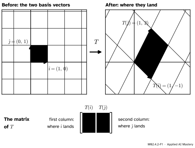
The matrix of a linear map is a record of two arrows. Its first column is where \(\ihat\) lands and its second column is where \(\jhat\) lands. The map is the module’s running example, \(T(x, y) = (x + y,\; -x + 2y)\).
Take the running example of this module, \(T(x, y) = (x + y,\; -x + 2y)\), and ask two questions.
Where does \(\ihat\) land? \(T(1, 0) = (1 + 0,\; -1 + 0) = (1, -1)\).
Where does \(\jhat\) land? \(T(0, 1) = (0 + 1,\; -0 + 2) = (1, 2)\).
Write each answer as a column and put the columns next to each other:
The first column is \(T(\ihat)\) and the second column is \(T(\jhat)\). Those four numbers hold the whole map. The yellow square in the figure shows why that is believable: the unit square is carried to the parallelogram with sides \(T(\ihat)\) and \(T(\jhat)\), and every other grid cell is a copy of it.
Build it up
Four numbers are only useful if they let us compute. Here is how to get \(T(\vect{v})\) for any \(\vect{v}\) out of the two columns, one small step at a time.
Step 1. Record the two landing spots. For our map they are \(T(\ihat) = (1, -1)\) and \(T(\jhat) = (1, 2)\). These are the columns of the matrix.
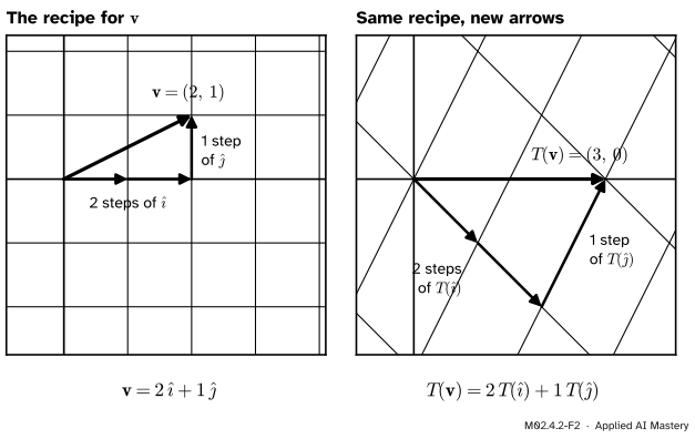
Step 2. Write the input as a recipe. Every vector is so many steps of \(\ihat\) plus so many steps of \(\jhat\). For \(\vect{v} = (2, 1)\) the recipe is \(\vect{v} = 2\,\ihat + 1\,\jhat\): the coordinates of a vector are its recipe.
Step 3. Keep the recipe, swap the arrows. A linear map sends a combination to the same combination of the images (Consequence 2 of the last lesson). So the image of \(\vect{v}\) uses the same numbers 2 and 1, with \(T(\ihat)\) in place of \(\ihat\) and \(T(\jhat)\) in place of \(\jhat\):
The map does not change the recipe, only the arrows it is made from. Two steps of \(\ihat\) and one of \(\jhat\) become two steps of \(T(\ihat)\) and one of \(T(\jhat)\).
That agrees with the formula, \(T(2, 1) = (2 + 1,\; -2 + 2) = (3, 0)\), but notice that we never used the formula. The two columns were enough.
Step 4. Give the calculation a name. “Take \(x\) of the first column plus \(y\) of the second column” is what multiplying a matrix by a vector means. We write it \(\mat{A}\vect{v}\).
Step 5. Read a matrix at a glance. Faced with any matrix, ask the same two questions: where does \(\ihat\) go (first column), and where does \(\jhat\) go (second column)?
\(\begin{bmatrix} 2 & 0 \\ 0 & 1 \end{bmatrix}\): \(\ihat\) lands on \((2, 0)\), twice as long, and \(\jhat\) stays at \((0, 1)\). The plane is stretched sideways.
\(\begin{bmatrix} 0 & -1 \\ 1 & 0 \end{bmatrix}\): \(\ihat\) lands on \((0, 1)\), where \(\jhat\) was, and \(\jhat\) lands on \((-1, 0)\). Both arrows have made a quarter turn anticlockwise.
\(\begin{bmatrix} 1 & 0 \\ 0 & 1 \end{bmatrix}\): both arrows stay where they are. This is the identity matrix, the map that moves nothing.
The next lesson builds a whole catalogue of maps this way.
The formal statement
NoteDefinition: matrix and matrix-vector product
A \(2 \times 2\)matrix is four numbers arranged in two rows and two columns. Its product with a vector \(\vect{v} = (x, y)\) is the combination of its columns that has the coordinates of \(\vect{v}\) as weights:
\[
\mat{A}\vect{v}
\;=\; \begin{bmatrix} a & b \\ c & d \end{bmatrix} \begin{bmatrix} \cdata{x} \\ \cdata{y} \end{bmatrix}
\;=\; \cdata{x} \cmodel{\begin{bmatrix} a \\ c \end{bmatrix}} + \cdata{y} \cmodel{\begin{bmatrix} b \\ d \end{bmatrix}} .
\]
The coordinates of the input say how much of each column to take. The columns are the images of the basis vectors. In displayed equations a vector is written as a column, which is why the landing spots stand upright in the matrix. The entry in row \(i\) and column \(j\) of a matrix is written \(a_{ij}\): row first, then column.
The row-by-row rule is the same thing. Carry out the scaling and the addition in the definition, one coordinate at a time:
\[
\begin{aligned}
x \begin{bmatrix} a \\ c \end{bmatrix} + y \begin{bmatrix} b \\ d \end{bmatrix}
&= \begin{bmatrix} xa \\ xc \end{bmatrix} + \begin{bmatrix} yb \\ yd \end{bmatrix} \\
&= \begin{bmatrix} ax + by \\ cx + dy \end{bmatrix} .
\end{aligned}
\]
The first step scales each column. The second adds, coordinate by coordinate. Look at the top entry, \(ax + by\). It uses only the top row \((a, b)\) of the matrix: multiply the row’s entries by the matching entries of \((x, y)\) and add. The bottom entry does the same with the bottom row \((c, d)\). This “row times vector” is the dot product of M02.3. So there are two ways to see one product. The column view says what the product means. The row view is a quick way to compute it entry by entry. They cannot disagree, because the second is the first written out.
NoteResult: matrices and linear maps of the plane are the same things
For every \(2 \times 2\) matrix \(\mat{A}\), the function \(\vect{v} \mapsto \mat{A}\vect{v}\) is a linear map.
Every linear map \(T\) of the plane is \(\vect{v} \mapsto \mat{A}\vect{v}\) for exactly one matrix \(\mat{A}\): the one whose columns are \(T(\ihat)\) and \(T(\jhat)\).
Proof of 1. Call the columns \(\vect{a}_1\) and \(\vect{a}_2\). Take vectors \(\vect{u} = (u_1, u_2)\) and \(\vect{v} = (v_1, v_2)\) and numbers \(p\) and \(q\). The vector \(p\vect{u} + q\vect{v}\) has coordinates \((pu_1 + qv_1,\; pu_2 + qv_2)\), so by the definition
The second step multiplies out and regroups. The third uses the definition again. This is the combined rule of the last lesson, so the map is linear.
Proof of 2. Let \(\mat{A}\) have columns \(T(\ihat)\) and \(T(\jhat)\). Consequence 4 of the last lesson says \(T(x, y) = x\,T(\ihat) + y\,T(\jhat)\), and the right-hand side is exactly \(\mat{A}\vect{v}\). So \(\mat{A}\) works. Now suppose some matrix \(\mat{B}\), with columns \(\vect{b}_1\) and \(\vect{b}_2\), also satisfies \(\mat{B}\vect{v} = T(\vect{v})\) for every \(\vect{v}\). Feed it \(\ihat = (1, 0)\):
In the same way \(\jhat = (0, 1)\) gives \(T(\jhat) = \vect{b}_2\). So \(\mat{B}\) has the same columns as \(\mat{A}\): there is only one matrix. The little calculation is worth remembering on its own: multiplying a matrix by \(\ihat\) picks out its first column, and by \(\jhat\) its second.
In any number of dimensions. Nothing above depends on the number two. A linear map \(T : \R^n \to \R^m\) takes vectors with \(n\) coordinates to vectors with \(m\) coordinates. \(\R^n\) has \(n\) basis vectors \(\vect{e}_1, \dots, \vect{e}_n\), where \(\vect{e}_j\) has a 1 in place \(j\) and 0 elsewhere. The matrix of \(T\) has one column for each of them, \(\vect{a}_j = T(\vect{e}_j)\), and each column has \(m\) entries. That makes \(m\) rows and \(n\) columns, an \(m \times n\) matrix, and
Here \((\mat{A}\vect{x})_i\) means entry \(i\) of the result. Every \(m \times n\) matrix defines a linear map from \(\R^n\) to \(\R^m\) in this way, and every linear map from \(\R^n\) to \(\R^m\) comes from exactly one \(m \times n\) matrix. Lesson M02.4.4 explores what happens when \(m \neq n\).
Go deeper: the same proof with n columns
Let \(\mat{A}\) be \(m \times n\) with columns \(\vect{a}_1, \dots, \vect{a}_n\), and define \(\mat{A}\vect{x} = x_1\vect{a}_1 + \cdots + x_n\vect{a}_n\).
Every matrix gives a linear map. The vector \(p\vect{u} + q\vect{v}\) has \(j\)-th coordinate \(pu_j + qv_j\), so
Every linear map has a matrix. Any \(\vect{x}\) in \(\R^n\) is \(x_1\vect{e}_1 + \cdots + x_n\vect{e}_n\). Applying the combined rule \(n - 1\) times gives \(T(\vect{x}) = x_1T(\vect{e}_1) + \cdots + x_nT(\vect{e}_n)\), which is \(\mat{A}\vect{x}\) for the matrix with columns \(T(\vect{e}_j)\).
Only one. If \(\mat{B}\vect{x} = T(\vect{x})\) for all \(\vect{x}\), put \(\vect{x} = \vect{e}_j\). Every term of \(\mat{B}\vect{e}_j\) is multiplied by 0 except the \(j\)-th, which is multiplied by 1, so \(\mat{B}\vect{e}_j = \vect{b}_j\). Hence \(\vect{b}_j = T(\vect{e}_j)\) for every \(j\).
One caution for later. “Exactly one matrix” assumes that coordinates are measured with the standard basis vectors. Measured with a different basis, the same map gets a different matrix. That is the subject of M02.9, Change of basis.
Worked example
Compute \(\mat{A}\vect{v}\) for \(\mat{A} = \begin{bmatrix} 1 & 1 \\ -1 & 2 \end{bmatrix}\) and \(\vect{v} = (3, 2)\), both ways.
M02.4.2-F3
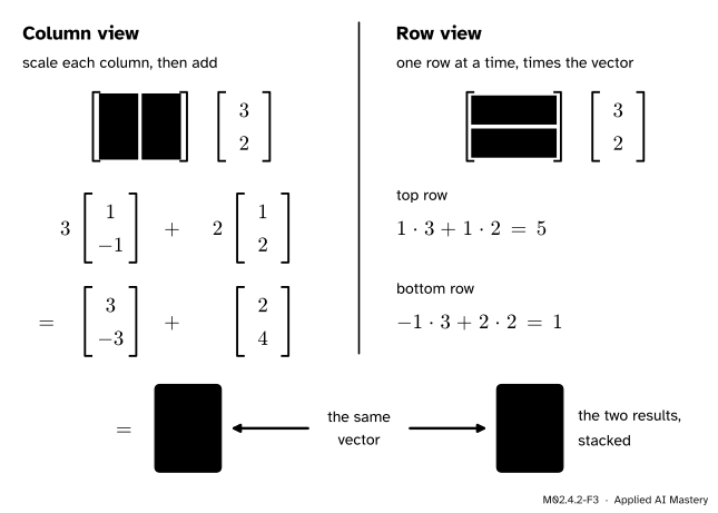
One product, two ways to see it. The column view combines the columns. The row view works out one entry of the answer at a time. Both give \((5, 1)\).
Column view. Take 3 of the first column and 2 of the second:
Row view. Top row times the vector: \(1 \cdot 3 + 1 \cdot 2 = 5\). Bottom row times the vector: \(-1 \cdot 3 + 2 \cdot 2 = 1\). Stack them: \((5, 1)\).
Check with the formula.\(T(3, 2) = (3 + 2,\; -3 + 4) = (5, 1)\). All three agree.
From a formula to its matrix. Find the matrix of \(S(x, y) = (3x - y,\; 2y)\). Ask the two questions. \(S(\ihat) = S(1, 0) = (3, 0)\) and \(S(\jhat) = S(0, 1) = (-1, 2)\), so
Compare the matrix with the formula. The first column, \((3, 0)\), collects everything that multiplies \(x\). The top row, \((3, -1)\), holds the coefficients of the first output, \(3x - 1y\). A quick test with \(\vect{v} = (1, 1)\): the columns give \(1\,(3, 0) + 1\,(-1, 2) = (2, 2)\), and the formula gives \(S(1, 1) = (3 - 1,\; 2) = (2, 2)\).
Code
First from scratch. A matrix is a list of rows, and each function is one of the two views.
def matvec_columns(A, v):"""Column view: add up v[j] times column j.""" m, n =len(A), len(A[0]) result = [0] * mfor j inrange(n): # one column at a timefor i inrange(m): # scale it by v[j] and add it on result[i] += v[j] * A[i][j]return resultdef matvec_rows(A, v):"""Row view: each entry of the answer is one row times the vector.""" result = []for row in A: total =0for a, x inzip(row, v): total += a * x result.append(total)return resultA = [[1, 1], [-1, 2]]print("column view:", matvec_columns(A, [3, 2]))print("row view: ", matvec_rows(A, [3, 2]))print("A times i-hat:", matvec_columns(A, [1, 0]), " A times j-hat:", matvec_columns(A, [0, 1]))
column view: [5, 1]
row view:    [5, 1]
A times i-hat: [1, -1]   A times j-hat: [1, 2]
The last line of output is the proof of uniqueness in action: multiplying by \(\ihat\) and \(\jhat\) returns the two columns. Now the library version. NumPy writes the product as A @ v.
import numpy as npA = np.array([[1, 1], [-1, 2]])v = np.array([3, 2])print("A @ v =", A @ v)print("columns of A:", A[:, 0], "and", A[:, 1])rng = np.random.default_rng(0)for _ inrange(1000): M, w = rng.normal(size=(2, 2)), rng.normal(size=2) by_columns = w[0] * M[:, 0] + w[1] * M[:, 1] by_rows = np.array([M[0] @ w, M[1] @ w])assert np.allclose(M @ w, by_columns) and np.allclose(M @ w, by_rows)print("column view = row view = @ on 1000 random matrices")
A @ v = [5 1]
columns of A: [ 1 -1] and [1 2]
column view = row view = @ on 1000 random matrices
Two near misses are worth seeing once, because NumPy runs both without complaint.
print("A * v =", (A * v).tolist()) # entry by entry: a table, not a vectorprint("v @ A =", (v @ A).tolist()) # combines the rows: a different map
A * v = [[3, 2], [-3, 4]]
v @ A = [1, 7]
The linear part of a neural-network layer is exactly W @ x, so these two slips are among the most common bugs in machine-learning code. The pitfalls below explain both.
Explore
M02.4-X1
Matrix playground
Drag the two round handles to choose where \(\ihat\) and \(\jhat\) land, and watch the grid follow. The read-out shows the matrix you have built and computes \(T(\vect{v})\) from its columns. Every handle also has a slider, so the keyboard works too.
Things to try:
Press This module’s T and drag \(\vect{v}\) to \((3, 2)\). Does the read-out give \((5, 1)\), as in the worked example? The tip of \(T(\vect{v})\) is just outside the picture, but the dashed path still shows the way: 3 of the first column, then 2 of the second.
Press Identity, then drag only \(T(\ihat)\). Which entries of the matrix change, and which grid lines move?
Slide \(T(\jhat)\) until it lies along the same line as \(T(\ihat)\). What happens to the yellow cell, and what does the area factor say?
Carry \(T(\jhat)\) across to the other side of \(T(\ihat)\). Watch the area factor change sign.
Press Play from identity to see the plane move from rest to your matrix.
Pitfalls
M02.4.2-F4
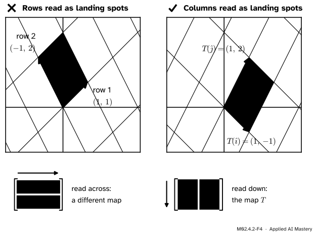
Wrong beside right. The same four numbers, read across instead of down, describe a different map with a different grid. The landing spots are the columns.
“The first row is where \(\ihat\) lands.”
We read text across, so the eye takes the rows first. For \(\begin{bmatrix} 1 & 1 \\ -1 & 2 \end{bmatrix}\) that gives \((1, 1)\) and \((-1, 2)\), which are not the landing spots. Test it: \(T(\ihat) = T(1, 0) = (1 + 0,\; -1 + 0) = (1, -1)\), the first column. Reading the rows gives the map of a different matrix, the one with rows and columns swapped. In NumPy the same slip is v @ A in place of A @ v. It combines the rows, and for \(\vect{v} = (3, 2)\) it returns \((1, 7)\) where the right answer is \((5, 1)\).
“To multiply, pair up the entries that sit in the same place.”
That is how vectors are added, not how a matrix acts. Entry-by-entry multiplication, A * v in NumPy, scales each column by its weight and then stops. It returns the table \(\begin{bmatrix} 3 & 2 \\ -3 & 4 \end{bmatrix}\), which is not a vector at all. The product finishes the job by adding those scaled columns: \((3, -3) + (2, 4) = (5, 1)\). Use @.
“A matrix can describe any map, if you pick the numbers well.”
Only linear ones. Whatever the four numbers are, \(\mat{A}\,\vect{0} = 0\,\vect{a}_1 + 0\,\vect{a}_2
= \vect{0}\), so the origin stays put. The shift \(S(x, y) = (x + 1, y)\) of the last lesson moves the origin, so no \(2 \times 2\) matrix can produce it. This is why a neural-network layer needs a separate bias vector: \(\mat{W}\vect{x} + \vect{b}\).
Check yourself
Recall
1. What do the two columns of a \(2 \times 2\) matrix record?
Show answer
Where the basis vectors land. The first column is \(T(\ihat)\) and the second is \(T(\jhat)\).
2. State the definition of \(\mat{A}\vect{v}\) for \(\vect{v} = (x, y)\) in words.
Show answer
Take \(x\) times the first column of \(\mat{A}\) plus \(y\) times the second column.
3. In the row view, how is the top entry of \(\mat{A}\vect{v}\) computed?
Show answer
Multiply the entries of the top row by the matching entries of \(\vect{v}\) and add: \(ax + by\).
4. What do you get when you multiply a matrix by \(\ihat\)? By \(\jhat\)?
Show answer
Its first column, and its second column.
5. How many \(2 \times 2\) matrices describe one given linear map of the plane?
Show answer
Exactly one: its columns are forced to be \(T(\ihat)\) and \(T(\jhat)\).
Exercises
1.★ Compute \(\begin{bmatrix} 2 & -1 \\ 1 & 3 \end{bmatrix}\begin{bmatrix} 4 \\ 1 \end{bmatrix}\) by the column view and by the row view.
Row view: top row \(2 \cdot 4 + (-1) \cdot 1 = 7\), bottom row \(1 \cdot 4 + 3 \cdot 1 = 7\). Both give \((7, 7)\).
2.★★ A linear map \(T\) of the plane sends \((1, 1)\) to \((3, 1)\) and \((1, -1)\) to \((1, 3)\). Find its matrix.
Show solution
We need \(T(\ihat)\) and \(T(\jhat)\). Write the basis vectors as combinations of the two inputs we know: \(\ihat = \tfrac12(1, 1) + \tfrac12(1, -1)\) and \(\jhat = \tfrac12(1, 1) - \tfrac12(1, -1)\). A linear map sends a combination to the same combination of the images, so
The matrix is \(\begin{bmatrix} 2 & 1 \\ 2 & -1 \end{bmatrix}\). Check: \(1\,(2, 2) + 1\,(1, -1) = (3, 1)\) and \(1\,(2, 2) - 1\,(1, -1) = (1, 3)\).
3.★★★ A matrix \(\mat{A}\) has first column \(\vect{a}_1 \neq \vect{0}\) and second column \(\vect{a}_2 = 2\vect{a}_1\). Show that every output \(\mat{A}\vect{v}\) lies on one line through the origin, and find every \(\vect{v}\) with \(\mat{A}\vect{v} = \vect{0}\).
Show solution
For \(\vect{v} = (x, y)\), \(\mat{A}\vect{v} = x\,\vect{a}_1 + y\,\vect{a}_2 = x\,\vect{a}_1 + 2y\,\vect{a}_1 = (x + 2y)\,\vect{a}_1\). Every output is a multiple of \(\vect{a}_1\), so it lies on the line through the origin in the direction \(\vect{a}_1\). The whole plane is squashed onto that line.
Since \(\vect{a}_1 \neq \vect{0}\), the output is \(\vect{0}\) exactly when \(x + 2y = 0\), that is \(x = -2y\). The solutions are \(\vect{v} = (-2s, s)\) for any number \(s\): a whole line of inputs is sent to the origin. Try it in the playground with the preset “Squash onto a line”, whose columns are \((1, 0.5)\) and \((2, 1)\).
Summary card
A matrix is where the basis vectors land, written as columns.
M02.4.2-F1
Columns are the landing spots.
Build it. First column \(T(\ihat)\), second column \(T(\jhat)\).
Use it (column view).\(\begin{bmatrix} a & b \\ c & d \end{bmatrix}\begin{bmatrix} x \\ y \end{bmatrix} = x\begin{bmatrix} a \\ c \end{bmatrix} + y\begin{bmatrix} b \\ d \end{bmatrix}\).
Compute it (row view). The same product is \((ax + by,\; cx + dy)\).
Why it is safe. Every matrix is a linear map, and every linear map has exactly one matrix.
In general. An \(m \times n\) matrix maps \(\R^n\) to \(\R^m\): \(\mat{A}\vect{x} = x_1\vect{a}_1 + \cdots + x_n\vect{a}_n\).
Sources and next steps
Sources. Each was opened and checked against this lesson on 12 November 2026.
Sheldon Axler, Linear Algebra Done Right, 4th edition (open access). Section 3C defines the matrix of a linear map (3.31) and notes that its \(k\)-th column is the map applied to the \(k\)-th standard basis vector. Result 3.50 states that a matrix times a column is a linear combination of the columns of the matrix. Result 3.71, in Section 3D, is the one-to-one correspondence between linear maps and matrices.
Grant Sanderson, Linear transformations and matrices, 3Blue1Brown, Linear Algebra, chapter 3. The source of the phrase and the picture: the columns of a matrix are where \(\ihat\) and \(\jhat\) land, and the product is \(x\) times the first column plus \(y\) times the second.
Marc Deisenroth, Aldo Faisal and Cheng Soon Ong, Mathematics for Machine Learning, Cambridge University Press, 2020 (free PDF). Section 2.7.1, Definition 2.19: the coordinates of the image of the \(j\)-th basis vector form the \(j\)-th column of the transformation matrix.
Gilbert Strang, Linear transformations and their matrices, MIT OpenCourseWare 18.06SC. A full lecture, with problems and solutions, on building the matrix of a linear transformation.