The outputs of a matrix are exactly the combinations of its columns. That set is the column space. Learn to picture it as a line, a plane or the whole space, decide whether Ax = b can be solved by asking whether b lies in it, and find its dimension, the rank, by counting pivots.
Describe the column space of a matrix as the set of all its outputs and as the span of its columns.
Decide whether Ax = b has a solution by testing whether b lies in the column space.
Find the rank of a matrix by elimination, and read off a basis of its column space from the pivot columns.
Explain why a product of matrices can reach no more than the matrix it applies last, and what that means for a narrow layer of a network.
In review. The maths and code on this page are checked by automated tests on every change, but an independent reader has not signed it off yet. Spot a mistake or a confusing step? Tell us.
The question
A network squeezes a 784-pixel image through a layer with only 2 units, then tries to rebuild all 784 pixels from those 2 numbers with one more matrix. However the weights are chosen, almost every image is out of reach of that last matrix. Which outputs can a matrix produce, and how do you measure how many there are?
From the last lesson
1. Which two equations must \(\mat{B}\) satisfy to be the inverse of \(\mat{A}\)?
Show answer
\(\mat{B}\mat{A} = \mat{I}\) and \(\mat{A}\mat{B} = \mat{I}\).
2. What is \((\mat{A}\mat{B})^{-1}\) in terms of \(\mat{A}^{-1}\) and \(\mat{B}^{-1}\)?
Show answer
\(\mat{B}^{-1}\mat{A}^{-1}\). The last map applied is the first one undone.
Intuition
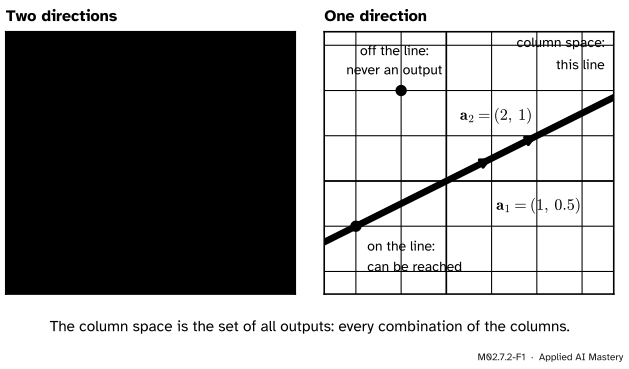
Multiplying a matrix by a vector combines its columns: \(\mat{A}\vect{x}\) is \(x_1\) of the first column plus \(x_2\) of the second, and so on (M02.4.2). Let \(\vect{x}\) run over every input and the outputs run over every combination of the columns: their span (M02.2). The span of the columns of a matrix is called its column space. It is everything the map can reach.
M02.7.2-F1
Left: the columns of the running matrix \(\mat{A}\) point in different directions and fill the plane. Right: the columns of the squash \(\mat{S}\) lie along one line and never leave it.
The left matrix is the running example \(\mat{A} = \begin{bmatrix} 1 & 1 \\ -1 & 2 \end{bmatrix}\). It is invertible (M02.7.1), so every target is reached. The right matrix is the squash \(\mat{S} = \begin{bmatrix} 1 & 2 \\ 0.5 & 1 \end{bmatrix}\), which is not. Now we can say what it misses: everything off one line.
Build it up
Step 1. “Can \(\vect{b}\) be reached?” is a question about the columns. The system \(\mat{A}\vect{x} = \vect{b}\) asks for weights that combine the columns into \(\vect{b}\): the column picture of M02.6.1. Try it on \(\mat{S}\). Every output is
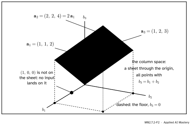
The three columns of \(\mat{B}\). The second repeats the direction of the first, so they span only a sheet: a plane through the origin.
The column \(\vect{a}_2\) is \(2\vect{a}_1\): no new direction. The columns \(\vect{a}_1\) and \(\vect{a}_3\) point in different directions, and two directions span a plane. Which plane? In each column the third entry is the sum of the first two, and adding or scaling such vectors keeps that property. So every output has \(b_3 = {b_1 + b_2}\). The point \((1, 0, 0)\) breaks the rule, so it is never an output.
Step 3. Count the directions. The dimension of the column space (M02.2.4) is called the rank of the matrix. So far: \(\mat{A}\) has rank 2, \(\mat{S}\) has rank 1, and \(\mat{B}\) has rank 2, although it has three columns.
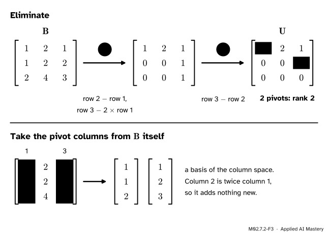
Step 4. Elimination counts for you. A hidden combination in a large matrix is hard to spot, but elimination (M02.6.2) finds it. For \(\mat{B}\): subtract row 1 from row 2, subtract twice row 1 from row 3, then subtract the new row 2 from row 3.
The pivots, in boxes, sit in columns 1 and 3. Those are the pivot columns. Column 2 has no pivot and is a free column. Two pivots, and the rank is 2.
Step 5. One more step makes the pattern plain. Make every pivot 1, and clear the entries above each pivot as well as below. Here that is one operation, row 1 minus row 2:
This is the reduced row echelon form, or reduced form. Its free column is twice its first pivot column, the same relation that holds in \(\mat{B}\).
The formal statement
NoteDefinitions: column space, subspace, rank
Let \(\mat{A}\) be an \({m \times n}\) matrix with columns \(\vect{a}_1, \dots, \vect{a}_n\).
Its column space is the set of all its outputs, \(\{\cmodel{\mat{A}\vect{x}} : \cdata{\vect{x}} \in \R^n\}\), which is the span of its columns. It is a set of vectors in \(\R^m\).
A set of vectors is a subspace if it contains \(\vect{0}\), and adding two of its vectors or scaling one of them always gives a vector of the set.
The rank of \(\mat{A}\) is the dimension of its column space.
In the plane the subspaces are the origin alone, the lines through the origin, and the whole plane. Space adds the planes through the origin.
The column space is a subspace. It contains \(\vect{0} = \mat{A}\vect{0}\). If \(\mat{A}\vect{x}\) and \(\mat{A}\vect{y}\) are two outputs, their sum is \({\mat{A}\vect{x} + \mat{A}\vect{y}} = {\mat{A}(\vect{x} + \vect{y})}\), an output. And \(c\,(\mat{A}\vect{x}) = \mat{A}(c\,\vect{x})\) is an output. Both are linearity (M02.4.1).
Solvability. The system \(\mat{A}\vect{x} = \vect{b}\) has a solution exactly when \(\vect{b}\) is in the column space of \(\mat{A}\): a solution is an input whose output is \(\vect{b}\).
NoteResult: pivot columns give the rank and a basis
Let \(\mat{R}\) be the reduced form of \(\mat{A}\). The columns of \(\mat{A}\) in the positions where \(\mat{R}\) has pivots form a basis of the column space of \(\mat{A}\). So the rank of \(\mat{A}\) is its number of pivots.
Proof. Call an equation \({x_1\vect{a}_1 + \dots + x_n\vect{a}_n} = \vect{0}\) a relation between the columns. It is the system \(\mat{A}\vect{x} = \vect{0}\) in the column picture.
Row operations keep every relation. A row operation never changes the solutions of a system (M02.6.2). So \(\mat{A}\vect{x} = \vect{0}\) and \(\mat{R}\vect{x} = \vect{0}\) have the same solutions: the columns of \(\mat{R}\) satisfy exactly the same relations as the columns of \(\mat{A}\), with the same weights.
In \(\mat{R}\) the relations are visible. A pivot of \(\mat{R}\) is a 1 with zeros above and below it. So if there are \(r\) pivots, the pivot columns are the basis vectors \(\vect{e}_1, \dots, \vect{e}_r\), which are independent. Now take a free column. Below the staircase every entry is zero, so its only non-zero entries \(f_1, \dots, f_k\) sit in the rows of the \(k\) pivots to its left. That makes it \({f_1\vect{e}_1 + \dots + f_k\vect{e}_k}\): a combination of the pivot columns to its left.
Carry both facts back to \(\mat{A}\). “Free column minus \(f_1\) of pivot column 1 minus \(\dots\) equals \(\vect{0}\)” is a relation in \(\mat{R}\), so by point 1 it holds in \(\mat{A}\): every free column of \(\mat{A}\) is a combination of the pivot columns of \(\mat{A}\). Free columns therefore add nothing to the span, and the pivot columns alone span the column space. They are also independent: a relation among them would, by point 1, be a relation among \(\vect{e}_1, \dots, \vect{e}_r\), which forces every weight to be zero.
Independent and spanning: a basis, of size the number of pivots. \(\blacksquare\)
Each row and each column holds at most one pivot, so for an \({m \times n}\) matrix
\[
\text{rank} \le m \qquad \text{and} \qquad \text{rank} \le n .
\]
A product reaches no more than the map it applies last. For any \(\vect{x}\), \((\mat{A}\mat{B})\vect{x} = \mat{A}(\mat{B}\vect{x})\), which is an output of \(\mat{A}\). So the column space of \(\mat{A}\mat{B}\) lies inside that of \(\mat{A}\). A basis of the smaller space is an independent set inside the larger one, and such a set is never bigger than the dimension of the space around it (M02.2.4). Hence \(\text{rank}(\mat{A}\mat{B}) \le \text{rank}(\mat{A})\).
That settles the opening question. The rebuilt image is \(\mat{W}_2(\mat{W}_1\vect{x})\), where \(\mat{W}_2\) has 784 rows and only 2 columns, so rank at most 2. Every rebuilt image lies on one plane through the origin of a 784-dimensional space. The plane is exact because the last step is one matrix. The non-linear functions of a real decoder (M02.5.4) bend it into a curved surface, still fixed by two numbers.
Go deeper: the rank of a product is at most the rank of either factor
The main text showed \(\text{rank}(\mat{A}\mat{B}) \le \text{rank}(\mat{A})\). The other half is \(\text{rank}(\mat{A}\mat{B}) \le \text{rank}(\mat{B})\).
Let \(\mat{B}\) have rank \(k\) and let \(\vect{v}_1, \dots, \vect{v}_k\) be a basis of its column space. Any output of \(\mat{B}\) is \({c_1\vect{v}_1 + \dots + c_k\vect{v}_k}\) for some numbers \(c_j\). So any output of \(\mat{A}\mat{B}\) is
by linearity. The column space of \(\mat{A}\mat{B}\) is therefore spanned by the \(k\) vectors \(\mat{A}\vect{v}_1, \dots, \mat{A}\vect{v}_k\). An independent set never outnumbers a spanning set (M02.2.4), so the dimension is at most \(k\). Each map in a chain can lose directions but never create them.
Frontier note: low rank on purpose: LoRA
To fine-tune a large language model, LoRA (Hu and others, 2021) freezes a weight matrix \(\mat{W}_0\), of shape \({d \times k}\), and learns only an update \(\mat{B}\mat{A}\), where \(\mat{B}\) is \({d \times r}\) and \(\mat{A}\) is \({r \times k}\) with \(r\) far smaller than \(d\) and \(k\) (Section 4.1 of the paper). By the result above the update has rank at most \(r\). The gain is in the count of numbers to train: \({r(d + k)}\) in place of \(dk\). With \(d = k = 4096\) and \(r = 8\) that is 65,536 in place of 16,777,216, a factor of 256.
Worked example
For the matrix \(\mat{B}\) above: (a) find the rank and a basis of the column space; (b) decide whether \(\vect{b} = (2, 3, 5)\) and \(\vect{b}' = (1, 0, 0)\) can be reached.
M02.7.2-F3
Elimination finds where the pivots are. The basis is read from the original matrix.
(a) Rank and basis. Step 4 found pivots in columns 1 and 3, so the rank is 2. A basis of the column space is columns 1 and 3 of \(\mat{B}\) itself: \((1, 1, 2)\) and \((1, 2, 3)\).
(b) The two targets. Run the same row operations on \(\mat{B}\) with a general target \((b_1, b_2, b_3)\) written beside it. The right-hand column becomes \(b_1\), then \({b_2 - b_1}\), and in the last row
The last row of \(\mat{U}\) is all zeros, so the last equation reads \(0 = {b_3 - b_1 - b_2}\). A target can be reached exactly when \(b_3 = {b_1 + b_2}\): the sheet of Step 2.
\(\vect{b} = (2, 3, 5)\): \(5 = {2 + 3}\), so it is reached. Row 2 of the eliminated system says \(x_3 = {b_2 - b_1} = 1\). Row 1 says \({x_1 + 2x_2 + x_3} = 2\). Choose \(x_2 = 0\), so \(x_1 = 1\). Check: \({(1, 1, 2) + (1, 2, 3)} = (2, 3, 5)\).
\(\vect{b}' = (1, 0, 0)\): \(0 \neq {1 + 0}\). The last equation would read \(0 = -1\). Not reached.
Code
Elimination from scratch, with exact fractions.
from fractions import Fractiondef echelon(A):"""Forward elimination. Returns the echelon form and the list of pivot columns (from 0).""" U = [[Fraction(x) for x in row] for row in A] rows, cols =len(U), len(U[0]) pivots, r = [], 0# r is the row where the next pivot will gofor c inrange(cols): usable = [i for i inrange(r, rows) if U[i][c] !=0]ifnot usable:continue# nothing to pivot on: column c is free U[r], U[usable[0]] = U[usable[0]], U[r]for i inrange(r +1, rows): factor = U[i][c] / U[r][c] U[i] = [x - factor * y for x, y inzip(U[i], U[r])] pivots.append(c) r +=1return U, pivotsdef rank(A):returnlen(echelon(A)[1])def reachable(A, b):"""Is b in the column space of A? Writing b beside A must not create a new pivot."""return rank([row + [x] for row, x inzip(A, b)]) == rank(A)B = [[1, 2, 1], [1, 2, 2], [2, 4, 3]]U, pivots = echelon(B)print("U =", [[int(x) for x in row] for row in U])print("pivot columns:", [c +1for c in pivots], " rank:", rank(B))print("basis of the column space:", [[row[c] for row in B] for c in pivots])print("(2, 3, 5) reachable:", reachable(B, [2, 3, 5]), " (1, 0, 0) reachable:", reachable(B, [1, 0, 0]))print("rank of A:", rank([[1, 1], [-1, 2]]), " rank of S:", rank([[1, 2], [Fraction(1, 2), 1]]))
U = [[1, 2, 1], [0, 0, 1], [0, 0, 0]]
pivot columns: [1, 3]   rank: 2
basis of the column space: [[1, 1, 2], [1, 2, 3]]
(2, 3, 5) reachable: True   (1, 0, 0) reachable: False
rank of A: 2   rank of S: 1
reachable uses the worked example: with \(\vect{b}\) written beside the matrix, a pivot appears in the last column exactly when some row reads “0 = something non-zero”.
The library call is np.linalg.matrix_rank. Here it measures the opening question’s bottleneck.
import numpy as npfrom numpy.linalg import matrix_rankprint("rank of B:", matrix_rank(np.array(B)))rng = np.random.default_rng(0)W1 = rng.normal(size=(2, 784)) # 784 numbers in, 2 outW2 = rng.normal(size=(784, 2)) # 2 numbers in, 784 outboth = W2 @ W1 # a 784 by 784 matrixprint("shape:", both.shape, " rank:", matrix_rank(both))
rank of B: 2
shape: (784, 784)   rank: 2
A matrix with 614,656 entries, and rank 2. Because rounding can turn an exact zero into a tiny number, matrix_rank counts the directions stretched by more than a small tolerance, using a method from M03.
Explore
The subspace viewer in lesson M02.7.4 draws the column space of a matrix you control. Press The running map, then Squash onto a line, and watch the plane collapse to a line. Drag one column off the line and the rank jumps back to 2.
Pitfalls
M02.7.2-F4
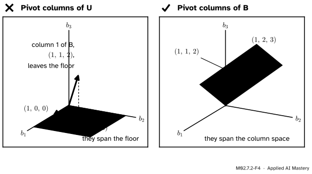
Wrong beside right. Columns 1 and 3 of the eliminated matrix \(\mat{U}\) span the floor. Columns 1 and 3 of \(\mat{B}\) itself span the column space.
“The pivot columns of the eliminated matrix are a basis of the column space.”
Row operations move the column space. Columns 1 and 3 of \(\mat{U}\) are \((1, 0, 0)\) and \((1, 1, 0)\). Both lie flat on the floor, but \((1, 1, 2)\), a column of \(\mat{B}\), does not. Elimination tells you which columns to take. Take them from the original matrix.
“The rank is the number of columns.”
It is the number of independent columns. \(\mat{B}\) has three non-zero columns and rank 2. In data work this happens whenever one feature is a combination of others, such as a total stored next to its parts. Extra columns do not guarantee reach either: \(\begin{bmatrix} 1 & 2 & 3 \\ 2 & 4 & 6 \end{bmatrix}\) has three columns, all along \((1, 2)\), and rank 1.
Check yourself
Recall
1. Describe the column space of a matrix in two ways.
Show answer
It is the set of all outputs \(\mat{A}\vect{x}\), and it is the span of the columns.
2. When does \(\mat{A}\vect{x} = \vect{b}\) have a solution?
Show answer
Exactly when \(\vect{b}\) lies in the column space of \(\mat{A}\).
3. What is the rank of a matrix?
Show answer
The dimension of its column space, which equals the number of pivots.
4. After elimination, which columns form a basis of the column space?
Show answer
The columns of the original matrix that stand where the pivots are.
5. What is the largest possible rank of a matrix with 5 rows and 3 columns? Can its columns reach all of \(\R^5\)?
Show answer
3, the number of columns. No: the column space has dimension at most 3, and \(\R^5\) has dimension 5.
Exercises
1.★ Let \(\mat{M} = \begin{bmatrix} 1 & 3 \\ 2 & 6 \end{bmatrix}\). Describe its column space and give its rank. Is \((2, 4)\) reached? Is \((1, 1)\)?
Show solution
The second column is 3 times the first, so the column space is the line through \((1, 2)\) and the rank is 1. \((2, 4) = 2\,(1, 2)\) is reached, for instance by \(\vect{x} = (2, 0)\). \((1, 1)\) is not a multiple of \((1, 2)\), so it is not.
2.★★ Let \(\mat{C} = \begin{bmatrix} 1 & 0 & 2 \\ 2 & 1 & 5 \\ 1 & 1 & 3 \end{bmatrix}\). (a) Find its rank and a basis of its column space. (b) Find the condition on \((b_1, b_2, b_3)\) for \(\mat{C}\vect{x} = \vect{b}\) to have a solution. (c) Is \((3, 4, 1)\) reached? Is \((1, 1, 1)\)?
Show solution
(a) Row 2 minus twice row 1 is \((0, 1, 1)\). Row 3 minus row 1 is \((0, 1, 1)\). Subtracting the new row 2 from the new row 3 gives \((0, 0, 0)\). The pivots are in columns 1 and 2, so the rank is 2 and a basis is columns 1 and 2 of \(\mat{C}\): \((1, 2, 1)\) and \((0, 1, 1)\).
(b) The same operations on the right-hand side give \(b_1\), then \({b_2 - 2b_1}\), then \({(b_3 - b_1) - (b_2 - 2b_1)}\), or \({b_3 + b_1 - b_2}\). The last row of zeros needs \({b_3 + b_1 - b_2} = 0\), that is, \(b_2 = {b_1 + b_3}\).
3.★★★ Suppose an \({m \times n}\) matrix \(\mat{A}\) has rank 1. (a) Show that there are a vector \(\vect{u}\) in \(\R^m\) and numbers \(v_1, \dots, v_n\) such that column \(j\) of \(\mat{A}\) is \(v_j\vect{u}\). (b) Deduce that the entry in row \(i\), column \(j\) is \(u_i v_j\), so \(\mat{A}\) is described by \({m + n}\) numbers, not \(mn\). (c) Write the squash \(\mat{S}\) in this form.
Show solution
(a) Rank 1 means the column space has a basis of one vector, \(\vect{u}\). Every column lies in the column space, so column \(j\) is \(v_j\vect{u}\) for some number \(v_j\).
(b) Entry \(i\) of the column \(v_j\vect{u}\) is \(v_j u_i\). So \(a_{ij} = u_i v_j\): the whole matrix is fixed by the \(m\) entries of \(\vect{u}\) and the \(n\) numbers \(v_j\).
(c) Take \(\vect{u} = (1, 0.5)\), the first column. The columns are \(1\,\vect{u}\) and \(2\,\vect{u}\), so \(v_1 = 1\) and \(v_2 = 2\). Check an entry: \(a_{22} = u_2 v_2 = {0.5 \cdot 2} = 1\).
Summary card
The column space is everything a matrix can reach, and the rank counts its directions.
M02.7.2-F1
A plane, or only a line.
Column space. All outputs \(\mat{A}\vect{x}\): the span of the columns. A subspace of \(\R^m\).
Solvability.\(\mat{A}\vect{x} = \vect{b}\) has a solution exactly when \(\vect{b}\) is in the column space.
Rank. The dimension of the column space: the number of pivots. At most \(m\) and at most \(n\).
Basis. The columns of the original matrix in the pivot positions.
Products.\(\text{rank}(\mat{A}\mat{B}) \le \text{rank}(\mat{A})\): a narrow layer limits everything after it.
Sources and next steps
Sources. Each was opened and checked against this lesson on 12 November 2026.
Sheldon Axler, Linear Algebra Done Right, 4th edition (open access). Section 3B: the range (3.16) is a subspace (3.18). Section 3C: column rank, at most \(\min\{m, n\}\) (3.52), and rank (3.58).
Gilbert Strang, MIT OpenCourseWare 18.06SC, lecture summaries of Column space and nullspace, Solving Ax = 0 and The four fundamental subspaces. Solvable exactly when \(\vect{b}\) is in the column space; rank equals the number of pivots; row operations affect the column space; the pivot columns form a basis of it.
Grant Sanderson, Inverse matrices, column space, and null space, 3Blue1Brown, Linear Algebra, chapter 7. Column space as the span of the columns; rank as the number of dimensions in it.
Marc Deisenroth, Aldo Faisal and Cheng Soon Ong, Mathematics for Machine Learning, Section 2.6.2. A basis of the column space comes from the pivot columns, and a system can be solved if and only if the augmented matrix has the same rank.
Edward Hu and others, LoRA: Low-Rank Adaptation of Large Language Models, arXiv, 2021. Section 4.1: the update to a frozen \({d \times k}\) weight matrix is \(\mat{B}\mat{A}\) with \(\mat{B}\) of shape \({d \times r}\), \(\mat{A}\) of shape \({r \times k}\) and \(r \ll \min(d, k)\).