How determinants are really computed: by elimination, as a product of pivots, in about n cubed over 3 steps. Then where the determinant appears in machine learning, as the factor that rescales a probability density, and why solvers avoid it.
Say what each row operation of elimination does to a determinant, and why.
Compute a determinant by reducing a matrix to triangular form and multiplying the pivots.
Compare the cost of elimination with the cost of cofactor expansion.
Use the determinant as the change-of-variables factor for a density under a linear map.
Explain why numerical code solves systems by elimination and reports log-determinants, not raw determinants.
In review. The maths and code on this page are checked by automated tests on every change, but an independent reader has not signed it off yet. Spot a mistake or a confusing step? Tell us.
The question
The cofactor rule finds a 3 by 3 determinant with a handful of multiplications. For a 25 by 25 matrix the same rule needs more than \(10^{25}\) products: at a billion a second, about 490 million years. NumPy returns the answer before your finger leaves the key. What does it do differently? And once determinants are that cheap, why do the libraries that solve linear systems still refuse to use them?
From the last lesson
1. Which three statements about a 2 by 2 matrix are always true together or false together?
Show answer
Its determinant is zero; its columns are linearly dependent (they lie on one line); it has no inverse.
2. State the product rule, and give the reason in one sentence.
Show answer
\({\det(\mat{A}\mat{B})} = {\det(\mat{A})\det(\mat{B})}\). Applying one map after another scales areas by one factor and then by the other, so the factors multiply.
Intuition
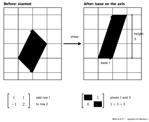
Elimination (lesson M02.6.2) has one main move: add a multiple of one row to another. Do it to the matrix of our map \(T\) and watch the parallelogram of its columns.
M02.8.4-F1
Adding row 1 to row 2 moves every point \({(x, y)}\) along a vertical line, to \({(x, y + x)}\). That is a shear. It slides the parallelogram until one side lies along the axis, and it does not change the area.
So elimination tidies the parallelogram for free. When it has finished, one side lies along the horizontal axis, and the area is simply base times height: \({1 \times 3 = 3}\). Those two numbers sit on the diagonal of the reduced matrix: they are the pivots.
That is how numerical libraries such as NumPy find the determinant of a large matrix: eliminate, then multiply the pivots.
Build it up
Step 1. A triangular matrix shows its determinant on its diagonal. For a 2 by 2 matrix with a zero below the diagonal, \({\det \begin{bmatrix} a & b \\ 0 & d \end{bmatrix}} = {ad - b \cdot 0} = ad\). For a 3 by 3 one, the cofactor rule gives
The same happens in any size. Expand down the first column: every entry below \(a_{11}\) is zero, so the determinant is \(a_{11}\) times the determinant of a smaller triangular matrix, and repeating the step works down the whole diagonal.
Step 2. Adding a multiple of one row to another changes nothing. In the 2 by 2 case,
\[
\begin{aligned}
& \det \begin{bmatrix} a & b \\ c + ka & d + kb \end{bmatrix} \\[4pt]
&\quad = a(d + kb) - b(c + ka) \\
&\quad = ad + kab - bc - kab \\
&\quad = ad - bc .
\end{aligned}
\]
Step 3. Swapping two rows reverses the sign.\({\det \begin{bmatrix} c & d \\ a & b \end{bmatrix}} = {cb - da} = {-(ad - bc)}\). A swap is a mirror.
Step 4. Put them together. Reduce the matrix to triangular form using only these two moves. Multiply the diagonal. Change the sign once for every swap you made.
Step 5. Count the work. Clearing the column under each pivot of an \(n\) by \(n\) matrix takes about \({n^3/3}\) multiplications in all (exercise 3 counts them). The cofactor rule, expanded all the way down, adds up \(n!\) products.
Size \(n\)
Cofactor rule: \(n!\) products
Elimination: steps
3
6
10
10
3,628,800
339
25
about \(1.55 \times 10^{25}\)
5,224
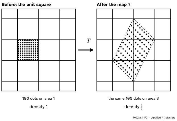
Step 6. A first use: densities. Scatter 100 dots evenly over the unit square and put them through \(T\).
M02.8.4-F2
The map does not create or destroy dots. It spreads the same 100 over three times the area, so there are a third as many per unit of area.
Replace “dots” by “probability” and you have the rule that machine learning uses whenever a model reshapes a random quantity: divide the density by the area factor.
Step 7. Why solvers still avoid determinants. There is a formula, Cramer’s rule, that solves \({\mat{A}\vect{x} = \vect{b}}\) using determinants only. For two equations it reads
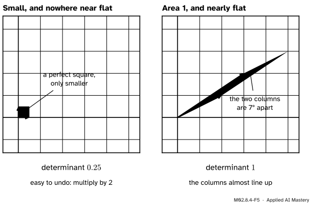
which is the inverse formula of lesson M02.7.1 applied to \(\vect{b}\). For \(n\) unknowns it needs \({n + 1}\) determinants, each as costly as the one elimination that already solves the system. Worse, a determinant is a product of \(n\) pivots, so for large \(n\) it is easily too large or too small for a computer to hold. And its size is a poor guide to trouble:
M02.8.4-F5
The matrix on the left has the smaller determinant, and it is the harmless one. The matrix on the right, with columns \({(2, 1)}\) and \({(3, 2)}\), has determinant exactly 1 while its columns nearly line up.
The formal statement
NoteResult: the determinant from elimination
Suppose elimination turns a square matrix \(\mat{A}\) into an upper triangular matrix \(\mat{U}\), using row replacements and \(s\) row swaps. Then
and by the product rule of the last lesson, \({\det \mat{U}} = {\det(\mat{E}_m) \cdots \det(\mat{E}_1) \det(\mat{A})}\). Two kinds of elementary matrix appear.
A row replacement is the identity matrix with one extra entry \(k\) below the diagonal. It is triangular with ones on its diagonal, so by Step 1 and the transpose rule its determinant is 1. In the plane it is the shear of the anchor figure.
A row swap is the identity matrix with two rows exchanged. The identity has determinant 1, and exchanging two rows reverses the sign, so its determinant is \({-1}\). Step 3 showed the sign change for 2 by 2 matrices, and exercise 3 of lesson M02.8.2 with the transpose rule shows it for the first two rows of a 3 by 3 one. It holds for any two rows in every size; we take that general fact on trust here.
Hence \({\det \mat{U} = (-1)^s \det \mat{A}}\). Multiply both sides by \({(-1)^s}\), and use \({(-1)^s(-1)^s = 1}\), to get \({\det \mat{A} = (-1)^s \det \mat{U}}\). Step 1 says that \(\det \mat{U}\) is the product of its diagonal entries. If a column has no pivot, a diagonal entry of \(\mat{U}\) is zero, the product is zero, and the matrix is singular.
NoteResult: the change-of-variables factor for a linear map
Let points be spread over the plane with density \(p\), an amount per unit area. Move every point \(\vect{x}\) to \({\vect{y} = \mat{A}\vect{x}}\), where \({\det \mat{A} \neq 0}\). The density of the moved points is
Derivation. Take a small square \(S\) around \(\vect{x}\), small enough that the density is nearly constant on it. It holds the amount \({p(\vect{x}) \times \text{area}(S)}\). The map carries exactly that amount onto the image of \(S\), whose area is \({\abs{\det \mat{A}} \times \text{area}(S)}\) by the first lesson of this module. Density is amount divided by area:
The absolute value appears because a flipped region still has positive area. In three dimensions the same argument runs with volumes. When the amount is probability, \(p\) and \(q\) are probability densities (module M06.6), and the factor is what keeps the total at 1.
A smooth map that is not linear still looks linear close to any one point. The matrix of that local linear map is called the Jacobian, and the same formula holds with its determinant in place of \(\det \mat{A}\). That needs calculus, and course M05 derives it.
Frontier note: normalising flows: models built on this factor
A normalising flow is a generative model that pushes simple noise through a chain of invertible maps until it looks like data. Training it needs the density of the output, and the formula above supplies it, with one determinant per map: equation (2) of the survey by Papamakarios and co-authors is \({p_x(\vect{x})} = {p_u(\vect{u})\,\abs{\det J_T(\vect{u})}^{-1}}\). A general \(D\) by \(D\) determinant costs on the order of \(D^3\) steps, as Step 5 found, which is too slow inside a training loop. So a large family of flows uses the trick of this lesson: its layers have triangular Jacobians, whose determinant is the product of the diagonal. Course DL06 builds one.
Worked example
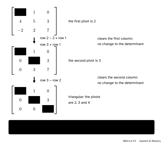
Find the determinant of \({\mat{K} = \begin{bmatrix} 2 & 1 & 0 \\ 4 & 5 & 3 \\ -2 & 2 & 7 \end{bmatrix}}\) by elimination.
M02.8.4-F3
Elimination on \(\mat{K}\). Every step is a row replacement, which leaves the determinant alone, so the determinant of the first matrix is the determinant of the last.
Clear the first column. The first pivot is 2. Subtract 2 times row 1 from row 2: \({(4, 5, 3)} - {2\,(2, 1, 0)} = {(0, 3, 3)}\). Add row 1 to row 3: \({(-2, 2, 7)} + {(2, 1, 0)} = {(0, 3, 7)}\).
Clear the second column. The second pivot is 3. Subtract row 2 from row 3: \({(0, 3, 7)} - {(0, 3, 3)} = {(0, 0, 4)}\).
Multiply the pivots. The matrix is now triangular with diagonal \({2, 3, 4}\), and no rows were swapped, so \({\det \mat{K}} = {2 \times 3 \times 4} = 24\).
A case that needs a swap. In \(\begin{bmatrix} 0 & 2 \\ 3 & 1 \end{bmatrix}\) the first pivot position holds a zero. Swap the rows to get \(\begin{bmatrix} 3 & 1 \\ 0 & 2 \end{bmatrix}\), which is triangular with diagonal product 6. One swap, so the determinant is \({-6}\). The formula agrees: \({0 \cdot 1 - 2 \cdot 3 = -6}\).
A density. Probability 1 is spread evenly over the unit square: density 1. After \(T\) it is spread evenly over a parallelogram of area 3, so the density there is \(\tfrac13\). A window of area \(0.6\) inside the parallelogram catches probability \({0.6 \times \tfrac13 = 0.2}\).
Code
From scratch. The function follows the recipe exactly, and counts its own multiplications and divisions.
def det_by_elimination(rows):"""Return (determinant, number of multiplications and divisions used).""" a = [[float(x) for x in row] for row in rows] n, sign, work =len(a), 1, 0for k inrange(n):if a[k][k] ==0: # no pivot here: look below for one below = [i for i inrange(k +1, n) if a[i][k] !=0]ifnot below:return0.0, work # a column with no pivot: singular a[k], a[below[0]] = a[below[0]], a[k] sign =-sign # a swap reverses the signfor i inrange(k +1, n): factor = a[i][k] / a[k][k] work +=1for j inrange(k +1, n): a[i][j] -= factor * a[k][j] # row i minus factor times row k work +=1 a[i][k] =0.0 product =1.0for k inrange(n): product *= a[k][k]return sign * product, work + n -1print(det_by_elimination([[2, 1, 0], [4, 5, 3], [-2, 2, 7]]))print(det_by_elimination([[0, 2], [3, 1]]))print(det_by_elimination([[1, 2], [0.5, 1]]))
(24.0, 10)
(-6.0, 3)
(0.0, 2)
The count for larger matrices, beside the number of products in a full cofactor expansion.
import mathimport randomrandom.seed(0)for n in (3, 10, 25): matrix = [[random.random() for _ inrange(n)] for _ inrange(n)] _, work = det_by_elimination(matrix)print(f"n = {n:2} cofactor products: {math.factorial(n):.3g} elimination steps: {work}")
n =  3   cofactor products: 6   elimination steps: 10
n = 10   cofactor products: 3.63e+06   elimination steps: 339
n = 25   cofactor products: 1.55e+25   elimination steps: 5224
The library version. np.linalg.det runs an elimination too. Because a product of many pivots can leave the range of numbers a computer can store, np.linalg.slogdet returns the sign and the logarithm of the size instead.
import numpy as npK = np.array([[2, 1, 0], [4, 5, 3], [-2, 2, 7]], dtype=float)print(round(np.linalg.det(K), 6))tiny =0.1* np.eye(500) # as easy to undo as a matrix can be: its inverse is 10 times the identitysign, log_size = np.linalg.slogdet(tiny)print(np.linalg.det(tiny), "|", sign, round(log_size, 2))flat = np.array([[1.0, 2.0, 3.0], [4.0, 5.0, 6.0], [7.0, 8.0, 9.0]]) # singular: row 3 - row 2 = row 2 - row 1print(abs(np.linalg.det(flat)) <1e-12, np.linalg.matrix_rank(flat))
24.0
0.0 | 1.0 -1151.29
True 2
The determinant of tiny is \({10^{-500}}\), far below the smallest number a 64-bit float can hold, so det returns 0.0 for a matrix that is perfectly invertible. slogdet reports the logarithm, about \({-1151.29}\), with no trouble. The last line shows the opposite hazard: that matrix is truly singular, but rounding can leave a tiny number such as 6.66e-16 in place of zero (the exact digits depend on the machine). Never test det(A) == 0. Ask for the rank, or just try to solve.
Last, the density rule, checked by simulation: 200,000 random points in the unit square, moved by \(T\), counted in a small window.
rng = np.random.default_rng(0)points = rng.random((200_000, 2)) # uniform on the unit square: density 1A = np.array([[1.0, 1.0], [-1.0, 2.0]])moved = points @ A.T # each row is A times a pointwindow = (np.abs(moved[:, 0] -1.0) <0.2) & (np.abs(moved[:, 1] -0.5) <0.2) # 0.4 by 0.4, inside the imagedensity = window.mean() /0.16print(round(density, 3), " predicted:", round(1/abs(np.linalg.det(A)), 3))
0.337 predicted: 0.333
Explore
The area explorer in lesson M02.8.2 lets you carry out the row operation of the anchor figure by hand. Press The course’s T: the read-out says \({+3.00}\). Now add row 1 to row 2, by raising the y of the first column from \({-1}\) to \(0\) and the y of the second from \(2\) to \(3\). The read-out says \({+3.00}\) again. Half-way, with one column moved, it said \({+2.00}\): a row operation moves both columns at once, and only the finished move is a shear.
Pitfalls
M02.8.4-F4
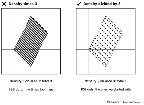
Wrong beside right. The map spreads 100 dots over 3 times the area. Multiplying the density by 3 would need 900 dots. Dividing it by 3 accounts for exactly the 100 there are.
“The map stretches space by 3, so the density is multiplied by 3.”
It is divided by 3. The same amount now lies on more area, so there is less of it per unit area. A quick test: the total, density times area, must not change. With density \(\tfrac13\) on area 3 the total is 1. With density 3 it would be 9.
“A tiny determinant means the matrix is nearly singular.”
Size is not shape. One tenth of the 500 by 500 identity has a determinant so small that it underflows to zero, and it is trivially invertible. The matrix with columns \({(2, 1)}\) and \({(3, 2)}\) has determinant 1 and columns that almost line up. How close a matrix is to collapse is measured by a different number, the condition number of module M03.8.
“To solve a system or test for an inverse in code, compute the determinant.”
Solving by Cramer’s rule repeats the work of elimination \({n + 1}\) times, and testing det(A) == 0 is defeated by rounding. Call a solver such as np.linalg.solve, which eliminates once and tells you if a pivot is missing. When a formula really needs the determinant, as a density does, use slogdet.
Check yourself
Recall
1. What does adding a multiple of one row to another do to the determinant, and what is the picture?
Show answer
Nothing. The operation is a shear, which slides a parallelogram along its base without changing its area.
2. What does swapping two rows do to the determinant?
Show answer
It reverses the sign and keeps the size.
3. What is the determinant of a triangular matrix?
Show answer
The product of the entries on its diagonal.
4. Points with density \(p\) are moved by a linear map with matrix \(\mat{A}\). What is their new density?
Show answer
\({p / \abs{\det \mat{A}}}\): the same amount spread over \(\abs{\det \mat{A}}\) times the area.
5. Why can np.linalg.det return 0.0 for a matrix that has an inverse, and what should you call instead?
Show answer
The determinant is a product of many pivots and can be too small for a floating-point number to hold. np.linalg.slogdet returns the sign and the logarithm of the size, which do fit.
Exercises
1.★ Find the determinant of \(\begin{bmatrix} 1 & 2 & 1 \\ 2 & 5 & 4 \\ 3 & 7 & 9 \end{bmatrix}\) by elimination.
Show solution
Row 2 minus 2 times row 1: \({(0, 1, 2)}\). Row 3 minus 3 times row 1: \({(0, 1, 6)}\). Row 3 minus the new row 2: \({(0, 0, 4)}\). The pivots are \({1, 1, 4}\) and no rows were swapped, so the determinant is \({1 \times 1 \times 4 = 4}\). Check by cofactors:
2.★★ Probability 1 is spread evenly over the unit square. Every point is moved by the matrix \(\begin{bmatrix} 2 & 0 \\ 1 & 3 \end{bmatrix}\). What is the density afterwards, and how much probability lies in a region of area \(1.5\) inside the image? What changes if the 3 is replaced by \({-3}\)?
Show solution
The determinant is \({2 \cdot 3 - 0 \cdot 1 = 6}\). The image is a parallelogram of area 6, and the density on it is \({1/6}\). A region of area \(1.5\) holds \({1.5 \times \tfrac16 = 0.25}\).
With \({-3}\) the determinant is \({-6}\). The map now turns the plane over, but its image is still a parallelogram of area 6 (the first one moved down by 3), and the density is \({1/\abs{-6} = 1/6}\) again. The sign does not affect a density.
3.★★★ Show that reducing an \(n\) by \(n\) matrix to triangular form takes \({(n^3 - n)/3}\) multiplications and divisions, when no pivot is zero.
Show solution
Take the pivot in column \(k\), for \({k = 1, \dots, n - 1}\). Below it are \({n - k}\) rows. For each of them we compute one factor (a division) and then update the \({n - k}\) entries to the right of the pivot column (one multiplication each). That is \({(n - k)(n - k + 1)}\) operations for column \(k\). Writing \({m = n - k}\), the total is
because both products in the bracket contain \({m(m+1)}\), and the factors left over differ by \({(m+2) - (m-1)} = 3\). When the terms are added, everything cancels except the last positive part and the first negative part, which is zero:
For \({n = 3}\) this is \(8\), and multiplying the three pivots adds 2 more, which is the count of 10 in the table.
Summary card
Eliminate, then multiply the pivots. A row replacement is a shear, and a shear changes no area.
M02.8.4-F1
Shear it straight, read the pivots.
Row replacement. No change to the determinant. Row swap. The sign reverses.
Recipe.\({\det \mat{A} = (-1)^s \times}\) the product of the pivots, with \(s\) the number of swaps.
Cost. About \({n^3/3}\) steps, against \(n!\) products for cofactors.
Densities. A linear map divides a density by \(\abs{\det \mat{A}}\).
In code. Solve with a solver, report slogdet, and never test det(A) == 0.
Sources and next steps
Sources. Each was opened and checked against this lesson on 12 November 2026.
Gilbert Strang, Properties of determinants, MIT OpenCourseWare 18.06SC, lecture summary. Properties 2 (a row exchange reverses the sign), 5 (a row replacement changes nothing) and 7 (a triangular matrix has the product of its pivots as determinant), and the remark that computers find determinants by elimination. The summary of the lecture on Cramer’s rule notes that computing inverses with Cramer’s rule is usually less efficient than using elimination.
Dan Margalit and Joseph Rabinoff, Interactive Linear Algebra, Section 4.1 (open textbook). The recipe for computing determinants by row reducing, with a factor \({(-1)^r}\) for \(r\) row swaps, and the remark that row reduction costs on the order of \(n^3\) operations, far fewer than cofactor expansion.
NumPy reference, numpy.linalg.det and numpy.linalg.slogdet. The determinant is computed by LU factorisation with the LAPACK routine getrf; slogdet exists because det may overflow or underflow, and its documentation uses the example of np.eye(500) * 0.1, with logarithm \({-1151.29}\).
Hossein Pishro-Nik, Introduction to Probability, Statistics, and Random Processes, Section 5.2.4 (open textbook). The method of transformations: the new joint density is the old one times the absolute value of the Jacobian determinant of the inverse map. For a linear map the inverse is \({\mat{A}^{-1}}\), so that factor is \({1/\abs{\det \mat{A}}}\), by the inverse rule of lesson M02.8.3.
George Papamakarios, Eric Nalisnick, Danilo Jimenez Rezende, Shakir Mohamed and Balaji Lakshminarayanan, Normalizing Flows for Probabilistic Modeling and Inference, Journal of Machine Learning Research 22(57), 2021. Equation (2) is the density formula of the frontier note; Section 3 gives the \(D^3\) cost and Section 3.1 the triangular Jacobians. Read in the arXiv version.
Next. Module M02.9 Change of basis asks how the matrix of a map changes when the grid itself is changed, and shows that the determinant does not change at all.