The null space of a matrix is the set of inputs it sends to zero. See why it is always a line, a plane or another subspace through the origin, compute it from the reduced form with free variables, and learn why every solution of Ax = b is one particular solution plus a vector of the null space.
Define the null space of a matrix and prove that it is a subspace of the input space.
Compute a basis of the null space from the reduced form: one special solution for each free variable.
Write every solution of Ax = b as one particular solution plus a vector of the null space.
Explain why two weight vectors that differ by a null-space vector of the data make identical predictions.
In review. The maths and code on this page are checked by automated tests on every change, but an independent reader has not signed it off yet. Spot a mistake or a confusing step? Tell us.
The question
Two models have different weights, yet they give exactly the same prediction on every example in the training set. No amount of that data can tell them apart. The cause is a set of directions that the data matrix sends to zero. What is that set, what shape does it have, and how do you find it?
From the last lesson
1. When does \(\mat{A}\vect{x} = \vect{b}\) have a solution?
Show answer
Exactly when \(\vect{b}\) lies in the column space of \(\mat{A}\).
2. After elimination, which columns form a basis of the column space?
Show answer
The columns of the original matrix that stand where the pivots are.
Intuition
The column space lives among the outputs. This lesson looks at the inputs. A matrix that squashes sends many inputs to each output, and the simplest output to ask about is \(\vect{0}\). The set of all inputs that a matrix sends to zero is called its null space.
M02.7.3-F1
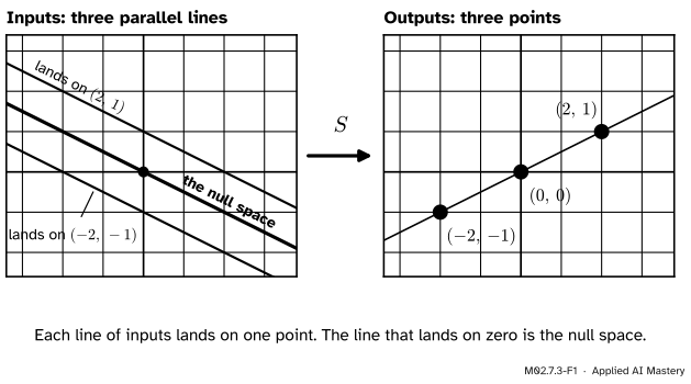
The squash \(\mat{S}\) of the last two lessons. Every input on the purple line is sent to \((0, 0)\): that line is the null space. Each parallel line is sent to a single point too.
Throughout this module the null space is drawn in purple, the colour this course uses for loss, because these are the inputs the map loses.
Where does the purple line come from? The squash is \(\mat{S} = \begin{bmatrix} 1 & 2 \\ 0.5 & 1 \end{bmatrix}\), and \(\mat{S}(x, y) = {(x + 2y)\,(1, 0.5)}\). The output is zero exactly when \({x + 2y} = 0\), which is the line through \((-2, 1)\). On the upper blue line \({x + 2y} = 2\), so every point lands on \(2\,(1, 0.5) = (2, 1)\).
Build it up
Step 1. Zero is always sent to zero. Every linear map fixes the origin (M02.4.1), so \(\vect{0}\) is in every null space. The question is whether anything else is.
Step 2. If one vector is lost, its whole line is lost.\(\mat{S}\) sends \(\vect{n} = (-2, 1)\) to zero. Then it sends \(3\vect{n} = (-6, 3)\) to \({3 \cdot \vect{0}} = \vect{0}\) too, and the same for every multiple. Sums behave the same way: zero plus zero is zero. A null space is never a scattering of points. It is the origin alone, a line, a plane or more.
Step 3. Moving along the null space cannot be seen from the output. Take any input \(\vect{x}\) and any \(\vect{n}\) in the null space. By linearity,
The output has not moved. That is why each blue line in the figure lands on one point: a blue line is the null space, shifted. M02.4.4 called \(\vect{n}\) a lost direction.
Step 4. Elimination finds the null space. The null space is the solution set of \(\mat{A}\vect{x} = \vect{0}\), and elimination solves systems. Take the \({2 \times 3}\) matrix of M02.4.4 and bring it to reduced form (M02.7.2) by subtracting twice row 2 from row 1:
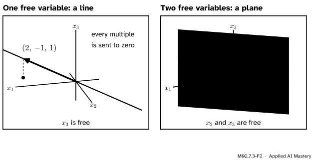
Columns 1 and 2 hold the pivots, so \(x_1\) and \(x_2\) are the pivot variables. Column 3 is free, so \(x_3\) is a free variable: it may take any value. The two rows of \(\mat{R}\) are the equations
Setting the free variable to 1 gives the special solution\((2, -1, 1)\), and the null space is the line through it. It is the lost direction that M02.4.4 found by inspection.
Step 5. Two free variables give a plane. Take the single row \(\begin{bmatrix} 1 & 2 & 0 \end{bmatrix}\), also from M02.4.4. It is already in reduced form, with one pivot. The pivot variable is \(x_1\) and both \(x_2\) and \(x_3\) are free. The one equation is \({x_1 + 2x_2} = 0\), so \(x_1 = -2x_2\) and
It is a set of vectors in \(\R^n\), the input space. Its dimension is called the nullity of \(\mat{A}\). Another name for the null space is the kernel.
The null space is a subspace. Check the three requirements of M02.7.2.
It contains \(\vect{0}\), because \(\mat{A}\vect{0} = \vect{0}\).
If \(\mat{A}\vect{u} = \vect{0}\) and \(\mat{A}\vect{v} = \vect{0}\), then \({\mat{A}(\vect{u} + \vect{v})} = {\mat{A}\vect{u} + \mat{A}\vect{v}}\), which is \({\vect{0} + \vect{0}} = \vect{0}\).
If \(\mat{A}\vect{u} = \vect{0}\) and \(c\) is a number, then \(\mat{A}(c\,\vect{u}) = c\,\mat{A}\vect{u} = c\,\vect{0} = \vect{0}\).
Row operations do not change it. A row operation never changes the solutions of a system (M02.6.2), and the null space is the solution set of \(\mat{A}\vect{x} = \vect{0}\). So \(\mat{A}\) and its reduced form \(\mat{R}\) have the same null space.
NoteResult: the special solutions span the null space
Let \(\mat{R}\) be the reduced form of \(\mat{A}\). For each free variable, build one special solution: set that free variable to 1, set the other free variables to 0, and read the pivot variables off \(\mat{R}\). Then the null space of \(\mat{A}\) is the set of all combinations of the special solutions.
Proof. In \(\mat{R}\) each pivot column is zero except for its pivot. So each non-zero row of \(\mat{R}\) is an equation that contains exactly one pivot variable:
Two things follow. Any choice of values for the free variables gives a solution: just set each pivot variable to minus the rest of its row. And two solutions with the same free values are the same solution, because the pivot variables are then forced.
Now take any solution \(\vect{x}\), with free values \(t_1, \dots, t_k\). Let \(\vect{s}_1, \dots, \vect{s}_k\) be the special solutions and form \(\vect{y} = {t_1\vect{s}_1 + \dots + t_k\vect{s}_k}\). It is a solution, because the null space is a subspace. Its free values are \(t_1, \dots, t_k\), because \(\vect{s}_j\) has a 1 in its own free position and 0 in the other free positions. So \(\vect{x}\) and \(\vect{y}\) are solutions with the same free values, and therefore \(\vect{x} = \vect{y}\). \(\blacksquare\)
NoteResult: every solution is a particular solution plus the null space
Suppose \(\vect{x}_p\) is one solution of \(\mat{A}\vect{x} = \vect{b}\). Then the solutions of \(\mat{A}\vect{x} = \vect{b}\) are exactly the vectors
\[
\cdata{\vect{x}_p} + \closs{\vect{n}}, \qquad \closs{\vect{n}} \text{ in the null space of } \mat{A}.
\]
Proof. Each such vector is a solution, by Step 3: \({\mat{A}(\vect{x}_p + \vect{n})} = {\vect{b} + \vect{0}} = \vect{b}\). Conversely, let \(\vect{x}\) be any solution. Then
so \(\vect{n} = {\vect{x} - \vect{x}_p}\) is in the null space, and \(\vect{x} = {\vect{x}_p + \vect{n}}\). \(\blacksquare\)
One particular solution says where the solutions are. The null space says what shape they make. Three things can be read off at once.
How many solutions. If \(\vect{b}\) is outside the column space there are none. If it is inside and the null space is only \(\{\vect{0}\}\), there is exactly one. If it is inside and the null space is bigger, there are infinitely many: a whole line of them or more. A linear system never has exactly two solutions (M02.6.3), and now the reason is geometric.
Independent columns. A vector \(\vect{x}\) in the null space is a relation \({x_1\vect{a}_1 + \dots + x_n\vect{a}_n} = \vect{0}\) between the columns. So the null space is \(\{\vect{0}\}\) exactly when the columns are independent (M02.2.3).
Models that cannot be told apart. Let \(\mat{X}\) be a table of data, one example in each row, and let a linear model predict \(\mat{X}\vect{w}\). If \(\mat{X}\vect{n} = \vect{0}\), then \({\mat{X}(\vect{w} + \vect{n})} = \mat{X}\vect{w}\): the weights \(\vect{w}\) and \({\vect{w} + \vect{n}}\) make the same prediction on every example. This happens whenever one feature is a combination of others.
Go deeper: a different particular solution gives the same set
The particular solution is not unique: any solution will do. Suppose \(\vect{x}_p\) and \(\vect{x}_q\) both solve \(\mat{A}\vect{x} = \vect{b}\). By the result above, \(\vect{x}_q = {\vect{x}_p + \vect{m}}\) for some \(\vect{m}\) in the null space. Then
and \({\vect{m} + \vect{n}}\) is again in the null space, because the null space is a subspace. So “\(\vect{x}_q\) plus the null space” is contained in “\(\vect{x}_p\) plus the null space”. Swapping the roles of the two solutions gives the reverse, so the two descriptions name the same set.
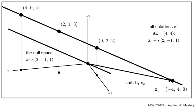
In the worked example below, the reduced form hands us \(\vect{x}_p = (-4, 4, 0)\). Starting from \((0, 2, 2)\) would describe the same line: the two differ by \(2\,(2, -1, 1)\).
Worked example
Find every solution of \(\mat{A}\vect{x} = (4, 4)\) for \(\mat{A} = \begin{bmatrix} 1 & 2 & 0 \\ 0 & 1 & 1 \end{bmatrix}\).
M02.4.4 found three inputs that land on \((4, 4)\). Now we find them all.
Reduce, with the target beside the matrix. Subtract twice row 2 from row 1:
The solutions of \(\mat{A}\vect{x} = (4, 4)\) form the blue line. It is the purple null space, moved from the origin to the particular solution \(\vect{x}_p\).
Putting \(s = 2\), \(3\) and \(4\) gives \((0, 2, 2)\), \((2, 1, 3)\) and \((4, 0, 4)\): the three inputs of M02.4.4.
Code
The reduced form from scratch, then the special solutions.
from fractions import Fractiondef rref(A):"""Reduced row echelon form. Returns it with the list of pivot columns (counted from 0).""" R = [[Fraction(x) for x in row] for row in A] rows, cols =len(R), len(R[0]) pivots, r = [], 0for c inrange(cols): usable = [i for i inrange(r, rows) if R[i][c] !=0]ifnot usable:continue# column c is free R[r], R[usable[0]] = R[usable[0]], R[r] R[r] = [x / R[r][c] for x in R[r]] # make the pivot 1for i inrange(rows):if i != r: # clear the column above and below it factor = R[i][c] R[i] = [x - factor * y for x, y inzip(R[i], R[r])] pivots.append(c) r +=1return R, pivotsdef null_space_basis(A):"""One special solution for each free variable.""" R, pivots = rref(A) n =len(R[0]) basis = []for free in [c for c inrange(n) if c notin pivots]: s = [Fraction(0)] * n s[free] = Fraction(1)for row, p inzip(R, pivots): # row k of R holds pivot k s[p] =-row[free] basis.append(s)return basisdef matvec(A, x):return [sum(a * b for a, b inzip(row, x)) for row in A]ints =lambda vectors: [[int(x) for x in v] for v in vectors]A = [[1, 2, 0], [0, 1, 1]]print("R =", ints(rref(A)[0]))print("null space of A :", ints(null_space_basis(A)))print("null space of (1 2 0):", ints(null_space_basis([[1, 2, 0]])))print("null space of B :", ints(null_space_basis([[1, 2, 1], [1, 2, 2], [2, 4, 3]])))print("null space of the running matrix:", null_space_basis([[1, 1], [-1, 2]]))
R = [[1, 0, -2], [0, 1, 1]]
null space of A      : [[2, -1, 1]]
null space of (1 2 0): [[-2, 1, 0], [0, 0, 1]]
null space of B      : [[-2, 1, 0]]
null space of the running matrix: []
The running matrix is invertible, so its list is empty. Now the worked example: a particular solution plus any multiple of the special solution.
x_p, n = [-4, 4, 0], [2, -1, 1]for s in (0, 2, 3, 4, -1.5): x = [p + s * d for p, d inzip(x_p, n)]print(f"s = {s:>4}: x = {x} -> A x = {matvec(A, x)}")
s =    0:  x = [-4, 4, 0]  ->  A x = [4, 4]
s =    2:  x = [0, 2, 2]  ->  A x = [4, 4]
s =    3:  x = [2, 1, 3]  ->  A x = [4, 4]
s =    4:  x = [4, 0, 4]  ->  A x = [4, 4]
s = -1.5:  x = [-7.0, 5.5, -1.5]  ->  A x = [4.0, 4.0]
The library version is scipy.linalg.null_space. Its basis vectors have length 1, so its answer is our special solution rescaled.
import numpy as npfrom scipy.linalg import null_spaceN = null_space(np.array(A, dtype=float))print("shape:", N.shape, " scaled so that the last entry is 1:", (N[:, 0] / N[2, 0]).round(12))X = np.array([[1, 2, 3], [2, 0, 2], [0, 1, 1], [3, 1, 4]]) # feature 3 = feature 1 + feature 2lost = np.array([1, 1, -1])w = np.array([1, 1, 1])print("X @ lost =", X @ lost)print("X @ w =", X @ w, " X @ (w + 2 lost) =", X @ (w +2* lost))
shape: (3, 1)   scaled so that the last entry is 1: [ 2. -1.  1.]
X @ lost     = [0 0 0 0]
X @ w        = [6 4 2 8]    X @ (w + 2 lost) = [6 4 2 8]
The weights \((1, 1, 1)\) and \((3, 3, -1)\) are different models with identical predictions: the opening question in four rows.
Explore
The subspace viewer in lesson M02.7.4 draws the null space of a matrix you control, in purple, in its left-hand panel. Press Squash onto a line and then Step x along the null space a few times. The input moves, and the output stays exactly where it was. Switch to a \({2 \times 3}\) matrix and the null space becomes a line in space, as in this lesson’s worked example.
Pitfalls
M02.7.3-F4
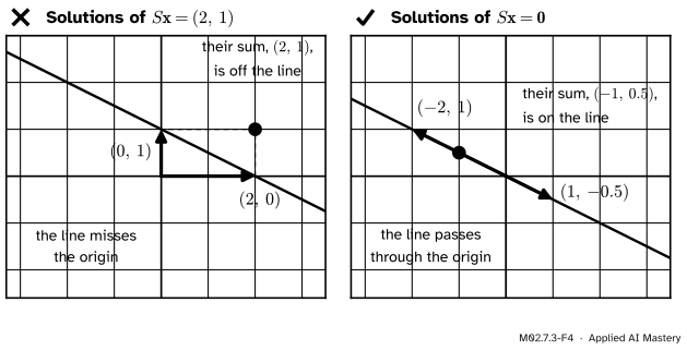
Wrong beside right. The solutions of \(\mat{S}\vect{x} = (2, 1)\) form a line, but it misses the origin and the sum of two solutions leaves it. Only for the target \(\vect{0}\) is the solution set a subspace.
“The solutions of \(\mat{A}\vect{x} = \vect{b}\) form a subspace.”
Only when \(\vect{b} = \vect{0}\). For any other target the zero vector is not a solution, since \(\mat{A}\vect{0} = \vect{0} \neq \vect{b}\), so the first requirement of a subspace already fails. The solution set has the shape of the null space, moved away from the origin.
“An invertible matrix has an empty null space.”
A null space is never empty. It always contains \(\vect{0}\). For an invertible matrix it contains nothing else: it is the set \(\{\vect{0}\}\), a single point, of dimension 0.
“The null space and the column space live in the same space.”
The null space is made of inputs, vectors in \(\R^n\). The column space is made of outputs, vectors in \(\R^m\). For the \({2 \times 3}\) matrix of the worked example, the null space is a line in space and the column space is the whole plane. Even for a square matrix, where both have the same number of entries, they are different sets.
“The special solution can be copied straight from the free column.”
The free column of \(\mat{R}\) in Step 4 is \((-2, 1)\), but the pivot variables are \(x_1 = 2\) and \(x_2 = -1\): moving a term across an equation flips its sign. Check a null vector by multiplying:
1. What is the null space of a matrix \(\mat{A}\)?
Show answer
The set of all inputs \(\vect{x}\) with \(\mat{A}\vect{x} = \vect{0}\). It is a subspace of the input space \(\R^n\).
2. Why is the zero vector in every null space?
Show answer
Because \(\mat{A}\vect{0} = \vect{0}\) for every matrix: a linear map fixes the origin.
3. How many special solutions does a matrix have?
Show answer
One for each free variable, that is, one for each column without a pivot.
4. If \(\vect{x}_p\) solves \(\mat{A}\vect{x} = \vect{b}\), what are all the solutions?
Show answer
\({\vect{x}_p + \vect{n}}\), where \(\vect{n}\) runs over the null space of \(\mat{A}\).
5. The null space of \(\mat{A}\) is \(\{\vect{0}\}\). How many solutions can \(\mat{A}\vect{x} = \vect{b}\) have?
Show answer
At most one: none if \(\vect{b}\) is outside the column space, exactly one if it is inside.
Exercises
1.★ Find the null space of \(\mat{M} = \begin{bmatrix} 1 & 3 \\ 2 & 6 \end{bmatrix}\).
Show solution
Subtract twice row 1 from row 2: the reduced form is \(\begin{bmatrix} 1 & 3 \\ 0 & 0 \end{bmatrix}\). The pivot variable is \(x_1\) and \(x_2\) is free. The one equation is \({x_1 + 3x_2} = 0\), so \(x_1 = -3x_2\). The special solution is \((-3, 1)\) and the null space is the line of its multiples. Check: \({-3\,(1, 2) + 1\,(3, 6)} = (0, 0)\).
2.★★ Let \(\mat{D} = \begin{bmatrix} 1 & 2 & 0 & 1 \\ 0 & 0 & 1 & 2 \end{bmatrix}\), which is already in reduced form. (a) Name the pivot and free variables. (b) Find the special solutions. (c) Find every solution of \(\mat{D}\vect{x} = (3, 4)\).
Show solution
(a) The pivots are in columns 1 and 3, so \(x_1\) and \(x_3\) are pivot variables and \(x_2\) and \(x_4\) are free.
(b) The equations are \({x_1 + 2x_2 + x_4} = 0\) and \({x_3 + 2x_4} = 0\), so \(x_1 = {-2x_2 - x_4}\) and \(x_3 = -2x_4\). With \(x_2 = 1\), \(x_4 = 0\): \((-2, 1, 0, 0)\). With \(x_2 = 0\), \(x_4 = 1\): \((-1, 0, -2, 1)\). Check the second: row 1 gives \({-1 + 0 + 0 + 1} = 0\) and row 2 gives \({-2 + 2} = 0\).
(c) Set both free variables to 0: \(x_1 = 3\) and \(x_3 = 4\), so \(\vect{x}_p = (3, 0, 4, 0)\). Every solution is
for any numbers \(s\) and \(t\): a plane inside \(\R^4\).
3.★★★ In a table of data \(\mat{X}\) with three features, the third feature of every example equals twice the first minus the second. (a) Find a non-zero vector in the null space of \(\mat{X}\). (b) A model has weights \(\vect{w} = (1, 2, 3)\). Describe all weight vectors that make the same predictions as \(\vect{w}\) on this data. (c) Find the one whose third weight is zero, and say what it means.
Show solution
(a) Write \(\vect{f}_1, \vect{f}_2, \vect{f}_3\) for the three columns. We are told \(\vect{f}_3 = {2\vect{f}_1 - \vect{f}_2}\), so \({2\vect{f}_1 - \vect{f}_2 - \vect{f}_3} = \vect{0}\). That is a relation between the columns, so \(\vect{n} = (2, -1, -1)\) satisfies \(\mat{X}\vect{n} = \vect{0}\).
So all the weights \({(1 + 2c,\; 2 - c,\; 3 - c)}\) make the same predictions. If the first two features are independent there are no others. Put \(\vect{f}_3 = {2\vect{f}_1 - \vect{f}_2}\) into a relation \({n_1\vect{f}_1 + n_2\vect{f}_2 + n_3\vect{f}_3} = \vect{0}\) and it becomes
which forces \(n_1 = -2n_3\) and \(n_2 = n_3\): a multiple of \((2, -1, -1)\).
(c) The third weight \({3 - c}\) is zero when \(c = 3\), which gives \((7, -1, 0)\). A model that ignores the third feature altogether predicts exactly as well on this data: the feature carries no information that the first two do not.
Summary card
The null space is everything a matrix sends to zero, and it shapes every solution set.
M02.7.3-F1
Each line lands on one point.
Null space. All \(\vect{x}\) with \(\mat{A}\vect{x} = \vect{0}\). A subspace of the input space \(\R^n\).
Invisible moves.\({\mat{A}(\vect{x} + \vect{n})} = \mat{A}\vect{x}\) for every \(\vect{n}\) in the null space.
Computing it. Reduce to \(\mat{R}\). One special solution for each free variable: that variable 1, the other free variables 0.
All solutions.\(\vect{x} = {\vect{x}_p + \vect{n}}\): one particular solution plus the null space.
In machine learning. Weights that differ by a null-space vector of the data predict identically.
Sources and next steps
Sources. Each was opened and checked against this lesson on 12 November 2026.
Sheldon Axler, Linear Algebra Done Right, 4th edition (open access). Section 3B: the definition of the null space (3.11), the null space is a subspace, with the three-part proof used here (3.13), and a linear map is injective exactly when its null space is \(\{0\}\) (3.15).
Grant Sanderson, Inverse matrices, column space, and null space, 3Blue1Brown, Linear Algebra, chapter 7. The set of vectors that land on the origin is called the null space or the kernel.
Marc Deisenroth, Aldo Faisal and Cheng Soon Ong, Mathematics for Machine Learning, Section 2.7.3. Definition 2.23 of the kernel, or null space, and the remark that it always contains the zero vector and is never empty.
SciPy manual, scipy.linalg.null_space. It constructs an orthonormal basis of the null space, returned as the columns of an array.