A linear map moves every point of the plane at once while keeping grid lines straight, parallel and evenly spaced. Learn the two rules behind that picture, test formulas against them, and see why two arrows are enough to pin a linear map down.
State the two rules, additivity and homogeneity, that make a function between vector spaces linear.
Recognise a linear map of the plane from its picture: grid lines stay straight, parallel and evenly spaced, and the origin stays put.
Test a formula for linearity, proving it when it passes and giving a counterexample when it fails.
Explain why a linear map is completely fixed by what it does to the basis vectors.
In review. The maths and code on this page are checked by automated tests on every change, but an independent reader has not signed it off yet. Spot a mistake or a confusing step? Tell us.
The question
Rotate a photo, stretch it, or slant it, and every straight edge in it stays straight. Bend it, and the edges curve. What exactly do the first three operations share that bending does not, and why is almost all of machine learning built out of that one shared property?
Intuition
A map (or transformation) is a function that takes a vector in and gives a vector out. Feed it every point of the plane and you can picture the whole plane moving at once: each point slides from where it was to where the map sends it.
Most ways of moving the plane make a mess of it. A linear map is the well-behaved kind. Draw the unit grid on the plane before the map, then look at where the grid ends up.
M02.4.1-F1
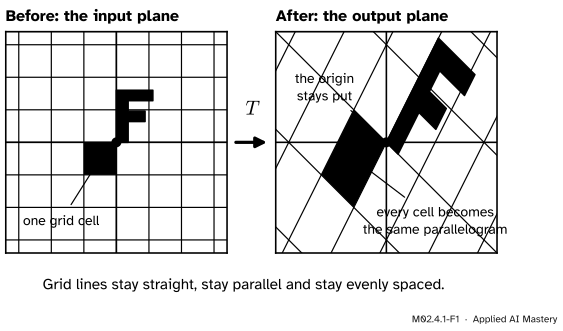
A linear map \(T\) moves the whole plane at once. The grid is distorted, but it is still a grid: its lines are straight, parallel and evenly spaced, and the origin has not moved. The map drawn here is \(T(x, y) = (x + y,\; -x + 2y)\), the running example of this module.
Three things are true of the picture on the right, and they are the whole idea:
Straight stays straight. No grid line has been bent.
Parallel and evenly spaced stay that way. Every grid cell has turned into the same parallelogram, so the grid still tiles the plane.
The origin stays put. The point \((0, 0)\) is sent to \((0, 0)\).
A rotation does this. So does a stretch, a slant (a shear) and a reflection. Bending does not, and neither does sliding the whole plane sideways, because that moves the origin.
Build it up
“The grid stays a grid” is a picture. To use it we need a rule we can check with algebra. The picture turns out to be the same thing as two short rules about adding and scaling, the only two operations vectors have.
Step 1. A map takes a vector to a vector. We write \(T(\vect{v})\) for the output when the input is \(\vect{v}\), and call it the image of \(\vect{v}\). For the map in the figure, \(T(2, 1) = (2 + 1,\; -2 + 2) = (3, 0)\).
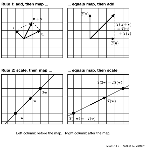
Step 2. Rule 1: adding survives the map. Take two vectors \(\vect{u}\) and \(\vect{v}\). You can add them first and then apply \(T\), or apply \(T\) to each and then add the results. For a linear map the two answers are always the same.
Step 3. Rule 2: scaling survives the map. Take a vector \(\vect{w}\) and a number \(c\). You can scale first and then apply \(T\), or apply \(T\) first and then scale. For a linear map the two answers are always the same.
M02.4.1-F2
The two rules, each shown before the map (left) and after it (right). Top: the image of a sum is the sum of the images, so a parallelogram is sent to a parallelogram. Bottom: the image of a multiple is the same multiple of the image, so evenly spaced points on a line are sent to evenly spaced points on a line.
Rule 1 is why parallel lines stay parallel: a parallelogram goes to a parallelogram. Rule 2 is why spacing stays even: the points \(\vect{w}, 2\vect{w}, 3\vect{w}, \dots\) go to \(T(\vect{w}), 2T(\vect{w}), 3T(\vect{w}), \dots\), which are equally spaced too. Together they force every straight line to land on a straight line, which we prove below.
The formal statement
NoteDefinition: linear map
A function \(T : \R^n \to \R^m\) is a linear map if, for all vectors \(\vect{u}, \vect{v}\) in \(\R^n\) and every real number \(c\), two rules hold.
\(\R^n\) is the set of all lists of \(n\) real numbers, so \(\R^2\) is the plane. The input and output spaces may have different dimensions; lesson M02.4.4 is about that. “Linear map”, “linear transformation” and “linear function” all mean the same thing.
Four consequences follow. Each is derived in full, because later lessons lean on every one.
Consequence 1: the origin stays put. Pick any vector \(\vect{v}\). The zero vector is \(0\,\vect{v}\), so
Why. If \(T\) is linear, then \(T(a\vect{u} + b\vect{v}) = T(a\vect{u}) + T(b\vect{v})\) by additivity, and that equals \(aT(\vect{u}) + bT(\vect{v})\) by homogeneity used twice. In the other direction, suppose the combined rule holds. Putting \(a = b = 1\) gives additivity. Putting \(b = 0\) gives \(T(a\vect{u}) = aT(\vect{u}) + 0\,T(\vect{v}) = aT(\vect{u})\), which is homogeneity.
In words: a linear map sends a linear combination to the same linear combination of the images.
Consequence 3: lines go to lines. A line is a set of points \(\vect{p} + s\,\vect{d}\), where \(\vect{p}\) is a point on it, \(\vect{d}\) is its direction and \(s\) runs over all real numbers. Apply \(T\) and use the combined rule with \(a = 1\), \(b = s\):
The right-hand side is again “a point plus \(s\) times a direction”: a line through \(T(\vect{p})\) with direction \(T(\vect{d})\). Three things can be read off it. The image is straight. Steps of equal size in \(s\) give equal steps along the image, so even spacing survives. And two parallel lines share a direction \(\vect{d}\), so their images share the direction \(T(\vect{d})\) and are parallel too, or are one and the same line. (If \(T(\vect{d}) = \vect{0}\), the whole line is squashed to the single point \(T(\vect{p})\). That is allowed, and lesson M02.4.4 returns to it.)
Consequence 4: two arrows fix everything. Write \(\ihat = (1, 0)\) and \(\jhat = (0, 1)\) for the two basis vectors of the plane. Any vector is a combination of them: \((x, y) = x\,\ihat + y\,\jhat\). The combined rule then gives
The input’s coordinates are untouched. All that the map contributes is the two images of the basis vectors. Know those two arrows and you know where every point goes. The next lesson writes those two arrows side by side and calls the result a matrix.
Go deeper: does additivity alone already force homogeneity?
Almost, and the gap is instructive. From additivity alone, \(T(2\vect{v}) = T(\vect{v} + \vect{v}) = 2T(\vect{v})\), and the same argument gives \(T(k\vect{v}) = kT(\vect{v})\) for every whole number \(k\). Writing \(\vect{v} = q \cdot \tfrac{1}{q}\vect{v}\) extends this to every fraction \(p/q\). So an additive map is automatically homogeneous for all rational scalars.
For irrational scalars such as \(\sqrt{2}\) it can fail. There are additive functions from \(\R\) to \(\R\) that are not of the form \(f(x) = ax\), but they are so irregular that their graphs are dense in the plane, and they cannot be written down by a formula: their existence relies on the axiom of choice. Any additive map that is also continuous is homogeneous. This is why the definition lists both rules: together they are exactly what is needed, with no extra assumption about continuity.
Worked example
Is \(T(x, y) = (x + y,\; -x + 2y)\) linear?
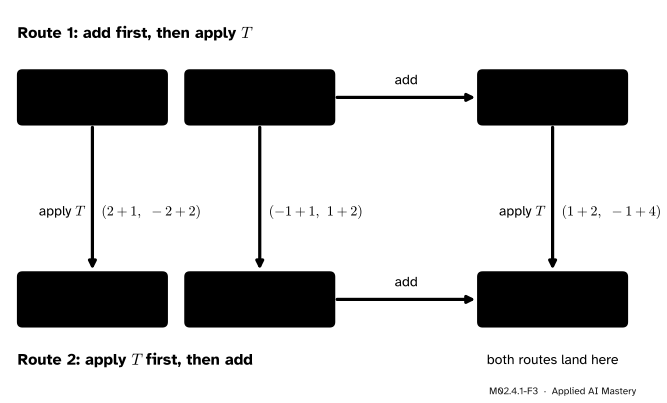
First, try numbers. Take \(\vect{u} = (2, 1)\) and \(\vect{v} = (-1, 1)\), and go both ways round.
M02.4.1-F3
Additivity checked with numbers. Route 1 adds first and applies \(T\) to the sum. Route 2 applies \(T\) to each vector and adds the results. Both routes end at \((3, 3)\).
Route 2: \(T(\vect{u}) = (2 + 1,\; -2 + 2) = (3, 0)\) and \(T(\vect{v}) = (-1 + 1,\; 1 + 2) = (0, 3)\), and their sum is \((3, 3)\). The routes agree.
Homogeneity with \(c = 2\): \(T(2\vect{u}) = T(4, 2) = (4 + 2,\; -4 + 4) = (6, 0)\), and \(2\,T(\vect{u}) = 2\,(3, 0) = (6, 0)\). They agree again.
Then prove it. Two agreeing examples are evidence, not proof. The definition says “for all”, so we need letters. Let \(\vect{u} = (u_1, u_2)\) and \(\vect{v} = (v_1, v_2)\), so that \(\vect{u} + \vect{v} = (u_1 + v_1,\; u_2 + v_2)\). Take one coordinate of the output at a time.
The first coordinate of \(T(\vect{u} + \vect{v})\) is the sum of the two inputs:
That is the second coordinate of \(T(\vect{u})\) plus the second coordinate of \(T(\vect{v})\). Both coordinates match, so \(T(\vect{u} + \vect{v}) = T(\vect{u}) + T(\vect{v})\).
For homogeneity, multiply the input by \(c\) and take the common factor out:
Both rules hold for all inputs, so \(T\) is linear. The proof worked because each output coordinate is a sum of plain multiples of the inputs: no squares, no products \(xy\), no added constants.
Two maps that fail.
\(S(x, y) = (x + 1,\; y)\) slides everything one unit to the right. Then \(S(0, 0) = (1, 0)\), which is not the origin, so by Consequence 1 it is not linear.
\(Q(x, y) = (x^2,\; y)\) keeps the origin, so that test is silent. Try homogeneity: \(Q(2 \cdot (1, 0)) = Q(2, 0) = (4, 0)\), but \(2\,Q(1, 0) = 2\,(1, 0) = (2, 0)\). They differ, so \(Q\) is not linear. One failing example is enough.
Code
First from scratch, with vectors as plain tuples, so that nothing is hidden.
def add(u, v):return (u[0] + v[0], u[1] + v[1])def scale(c, v):return (c * v[0], c * v[1])def T(v):"""The map from the worked example.""" x, y = vreturn (x + y, -x +2* y)u, v = (2, 1), (-1, 1)print("add, then map:", T(add(u, v)))print("map, then add:", add(T(u), T(v)))print("scale, then map:", T(scale(2, u)), " map, then scale:", scale(2, T(u)))
add, then map: (3, 3)
map, then add: (3, 3)
scale, then map: (6, 0)   map, then scale: (6, 0)
The outputs match the figure. Now the same idea with NumPy, turned into a tester that throws a thousand random inputs at any function.
import numpy as npdef looks_linear(f, n=2, trials=1000, seed=0):"""Check additivity and homogeneity on random inputs. A failure is a disproof.""" rng = np.random.default_rng(seed)for _ inrange(trials): u, v = rng.normal(size=n), rng.normal(size=n) a, b = rng.normal(size=2)ifnot np.allclose(f(a * u + b * v), a * f(u) + b * f(v)):returnFalsereturnTrueT =lambda p: np.array([p[0] + p[1], -p[0] +2* p[1]]) # the worked exampleS =lambda p: np.array([p[0] +1, p[1]]) # slides the planeQ =lambda p: np.array([p[0] **2, p[1]]) # squares a coordinatefor name, f in [("T", T), ("S", S), ("Q", Q)]:print(name, "passes"if looks_linear(f) else"fails")
T passes
S fails
Q fails
The tester uses the combined rule from Consequence 2, so one line checks both properties. Read its verdicts with care. “Fails” is certain: the tester found a counterexample. “Passes” only means no counterexample turned up in a thousand tries. The proof is the algebra in the worked example.
Explore
This module’s interactive, the matrix playground, lives in the next lesson, once you know that dragging two arrows is the same as choosing a matrix.
Pitfalls
M02.4.1-F4
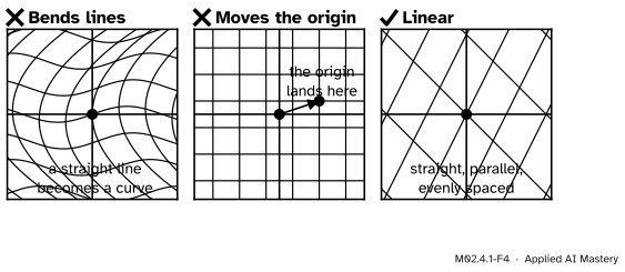
Wrong beside right. The first map bends lines. The second keeps every line straight but moves the origin. Only the third is linear.
“Its graph is a straight line, so it is linear.”
In school, \(f(x) = 2x + 3\) is called a linear function. In linear algebra it is not a linear map, because \(f(0) = 3 \neq 0\). A linear map plus a constant shift is called an affine map. The distinction matters all through machine learning: a neural-network layer computes \(\mat{W}\vect{x} + \vect{b}\), which is affine. Only the \(\mat{W}\vect{x}\) part is linear.
“I checked an example and it worked, so the map is linear.”
Examples can only disprove. The map \(Q(x, y) = (x^2, y)\) passes additivity for \(\vect{u} = (1, 0)\) and \(\vect{v} = (0, 1)\), since \(Q(1, 1) = (1, 1) = Q(1, 0) + Q(0, 1)\), yet it is not linear. To prove linearity, work with letters.
“A linear map must be reversible.”
Nothing in the two rules says so. The map \(P(x, y) = (x, 0)\) flattens the whole plane onto the horizontal axis. It is linear (check the rules) and it cannot be undone. Even the map that sends every vector to \(\vect{0}\) is linear.
Check yourself
Recall
1. What are the two rules that define a linear map?
Show answer
Additivity, \(T(\vect{u} + \vect{v}) = T(\vect{u}) + T(\vect{v})\), and homogeneity, \(T(c\vect{v}) = cT(\vect{v})\), for all vectors and all numbers \(c\).
2. In the grid picture, what three things stay true after a linear map of the plane?
Show answer
Grid lines stay straight, they stay parallel and evenly spaced, and the origin stays where it is.
3. Where does every linear map send the zero vector, and which rule shows it?
Show answer
To the zero vector. Homogeneity with \(c = 0\) gives \(T(\vect{0}) = T(0\vect{v}) = 0\,T(\vect{v}) = \vect{0}\).
4. Why is \(f(x) = 2x + 3\) not a linear map, and what is it called?
Show answer
Because \(f(0) = 3\), not \(0\). It is an affine map: a linear map followed by a shift.
5. To know where a linear map of the plane sends every point, how many outputs do you need to know?
Show answer
Two: \(T(\ihat)\) and \(T(\jhat)\). Then \(T(x, y) = x\,T(\ihat) + y\,T(\jhat)\).
Exercises
1.★ A linear map has \(T(\ihat) = (3, 1)\) and \(T(\jhat) = (-1, 2)\). Find \(T(2, 5)\).
2.★★ For each map, decide whether it is linear. Prove it or give a counterexample. (a) \(A(x, y) = (3x - y,\; 2y)\) (b) \(B(x, y) = (xy,\; x)\) (c) \(C(x, y) = (x,\; y - 4)\).
Show solution
(a) Linear. Each output is a sum of plain multiples of \(x\) and \(y\), and the proof in the worked example goes through coordinate by coordinate. For the first coordinate,
(c) Not linear. \(C(0, 0) = (0, -4)\), which is not the origin.
3.★★★ Let \(T\) be a linear map of the plane. Show that \(T\) sends the midpoint of any segment to the midpoint of the image segment.
Show solution
The midpoint of the segment from \(\vect{p}\) to \(\vect{q}\) is \(\tfrac12\vect{p} + \tfrac12\vect{q}\). By the combined rule with \(a = b = \tfrac12\), \(T(\tfrac12\vect{p} + \tfrac12\vect{q}) = \tfrac12 T(\vect{p}) + \tfrac12 T(\vect{q})\), which is the midpoint of the segment from \(T(\vect{p})\) to \(T(\vect{q})\). The same argument with \(a = 1 - s\), \(b = s\) shows that every point a fraction \(s\) of the way along a segment stays a fraction \(s\) of the way along its image.
Quick rejection. If \(T(\vect{0}) \neq \vect{0}\), the map is not linear.
Two arrows fix everything.\(T(x, y) = x\,T(\ihat) + y\,T(\jhat)\).
Sources and next steps
Sources. Each was opened and checked against this lesson on 12 November 2026.
Sheldon Axler, Linear Algebra Done Right, 4th edition (open access). Section 3A gives the definition of a linear map (3.1), with additivity and homogeneity under those names, and the linear map lemma (3.4): a linear map is fixed by its values on a basis.
Grant Sanderson, Linear transformations and matrices, 3Blue1Brown, Linear Algebra, chapter 3. The source of the grid picture: lines remain lines, the origin stays fixed, grid lines stay parallel and evenly spaced.