A linear system has no solution, exactly one, or infinitely many, and elimination tells you which. Learn to read the three cases from the last rows of the matrix, describe a whole line of solutions with a free variable, and prove that exactly two solutions can never happen.
Tell from the rows left by elimination whether a system has no solution, one solution or infinitely many.
Identify pivot columns and free variables in an echelon form.
Write the general solution of a system with a free variable as one solution plus a multiple of a direction.
Prove that a linear system with two different solutions has infinitely many.
In review. The maths and code on this page are checked by automated tests on every change, but an independent reader has not signed it off yet. Spot a mistake or a confusing step? Tell us.
The question
The system of the last lesson had exactly one solution. Some systems have none. Others have infinitely many: when a linear model has more weights than data points and fits its data perfectly, it can do so in endlessly many ways. How does elimination tell these cases apart, and why is there never a system with exactly two solutions?
From the last lesson
1. Name the three row operations.
Show answer
Swap two rows. Scale a row by a non-zero number. Replace a row by itself plus a multiple of another row.
2. Why does a row operation never change the solution set?
Show answer
Any vector that solves the old system solves the new one, and each operation can be undone by an operation of the same kind, so any vector that solves the new system solves the old one too.
Intuition
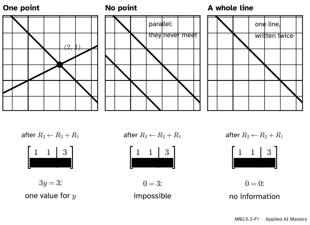
Draw two lines in a plane. Only three things can happen. They cross at one point, or they are parallel and never meet, or they are the same line drawn twice. Two equations in two unknowns are two lines (as long as each one really contains an unknown), so the system has one solution, no solution, or a whole line of solutions.
Elimination finds out which, without a drawing. The three systems below share their first row, \(x + y = 3\). Their second rows are \(-x + 2y = 0\), then \(-x - y = 0\), then \(-x - y = -3\). The same operation, \({R_2 \leftarrow R_2 + R_1}\), is applied to each.
M02.6.3-F1
Two lines can meet once, never, or everywhere. After one row operation, the last row of the matrix says which: a pivot, an impossible equation, or an equation that says nothing.
The whole lesson is in the last rows of those three matrices.
Build it up
Step 1. Read the last row.
In the first system the last row is \({[\,0 \;\; 3 \mid 3\,]}\), which says \(3y = 3\). There is a pivot, so \(y = 1\), and back substitution gives \(x = 2\). One solution.
In the second the last row is \({[\,0 \;\; 0 \mid 3\,]}\), which says \(0x + 0y = 3\). No choice of \(x\) and \(y\) makes \(0\) equal to \(3\). No solution. Elimination did not create this contradiction. It was there from the start: the original equations demand \(x + y = 3\) and \(x + y = 0\) at once.
In the third the last row is \({[\,0 \;\; 0 \mid 0\,]}\), which says \(0 = 0\). That is true for every \(x\) and \(y\), so the row rules nothing out. The second equation was the first one multiplied by \(-1\), and it carried no information of its own.
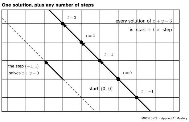
Step 2. One equation, two unknowns. The third system has come down to the single equation \(x + y = 3\). Column 1 has a pivot. Column 2 has none, so nothing pins \(y\) down. Call \(y\) a free variable and let it be any number \(t\). The equation then fixes \(x = 3 - t\). Every solution has the form
The general solution of \(x + y = 3\). Start at the solution \((3, 0)\) and take \(t\) steps of \((-1, 1)\). Each value of \(t\) gives one solution, and every solution arises this way.
Step 3. What the step is. The step \((-1, 1)\) is not itself a solution: \(-1 + 1 = 0\), not 3. It solves the same system with zeros on the right, \(x + y = 0\) and \(-x - y = 0\). Moving along it does not change the left-hand sides, and that is why adding it to a solution gives another solution.
The formal statement
Forward elimination, as in lesson M02.6.2, needs one extra rule. If a column has no non-zero entry to use as a pivot, at or below the current row, leave that column and move right. The result is an echelon form: each non-zero row begins further to the right than the row above it, and any rows of zeros are at the bottom.
NoteDefinition: pivot columns and free variables
In an echelon form, the first non-zero entry of each non-zero row is a pivot. A column that holds a pivot is a pivot column. An unknown whose column holds no pivot is a free variable.
NoteResult: the three cases
Let \({[\,\mat{U} \mid \vect{c}\,]}\) be an echelon form of \({[\,\mat{A} \mid \vect{b}\,]}\), for a system with \(n\) unknowns.
If some row is \({[\,0 \;\cdots\; 0 \mid c\,]}\) with \(c \neq 0\), there is no solution.
If there is no such row and all \(n\) columns of \(\mat{U}\) are pivot columns, there is exactly one solution.
If there is no such row and at least one unknown is free, there are infinitely many solutions.
Why. Row operations keep the solution set (lesson M02.6.2), so it is enough to count the solutions of the echelon system.
Case 1. The row says \(0 = c\) with \(c \neq 0\). That is false for every \(\vect{x}\).
Case 2. Rows of zeros say \(0 = 0\) and can be dropped. What is left is a triangular system with \(n\) pivots, and back substitution computes each unknown in exactly one way.
Case 3. Give each free variable any value you like. Then work up from the last non-zero row. Each row has a pivot, and it fixes that pivot’s unknown in exactly one way from values already chosen or found. So every choice of the free variables gives one solution, different choices give different solutions, and there are infinitely many choices.
The three cases cover every possibility. So no linear system has exactly two solutions, or exactly seventeen. There is also a direct proof, which shows where the infinitely many solutions come from.
NoteResult: never exactly two
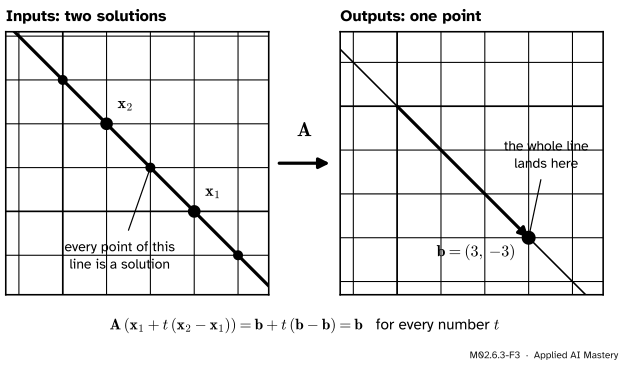
If \(\vect{x}_1\) and \(\vect{x}_2\) are two different solutions of \(\mat{A}\vect{x} = \vect{b}\), then every point of the line through them is a solution.
Proof. The points of the line through \(\vect{x}_1\) and \(\vect{x}_2\) are \(\vect{x}_1 + t\,{(\vect{x}_2 - \vect{x}_1)}\), one for each real number \(t\). Multiplying by a matrix is a linear map (lesson M02.4.2), so it can be applied term by term and the number \(t\) can be taken outside:
The second equality uses \(\mat{A}\vect{x}_1 = \vect{b}\) and \(\mat{A}\vect{x}_2 = \vect{b}\). So every point of the line is a solution. Two different values \(s\) and \(t\) give two different points, because the points differ by \({(t - s)}{(\vect{x}_2 - \vect{x}_1)}\), and neither factor is zero. There are infinitely many values of \(t\), so there are infinitely many solutions. \(\blacksquare\)
M02.6.3-F3
The proof as a picture, for the matrix with rows \((1, 1)\) and \((-1, -1)\). Two inputs that land on \(\vect{b}\) drag the whole line through them along, because the map sends the direction \(\vect{x}_2 - \vect{x}_1\) to zero.
The proof also shows the shape of a solution set. The difference of two solutions satisfies \(\mat{A}{(\vect{x}_2 - \vect{x}_1)} = \vect{b} - \vect{b} = \vect{0}\). So all solutions are reached from one particular solution by adding solutions of \(\mat{A}\vect{x} = \vect{0}\). Written out with one parameter for each free variable, this is the general solution. Lesson M02.7.3 gives the solutions of \(\mat{A}\vect{x} = \vect{0}\) a name, the null space.
Worked example
Solve
\[
\begin{aligned}
x + y + 2z &= 3 \\
2x + 3y + 5z &= 7 \\
x + 2y + 3z &= 4 .
\end{aligned}
\]
M02.6.3-F4
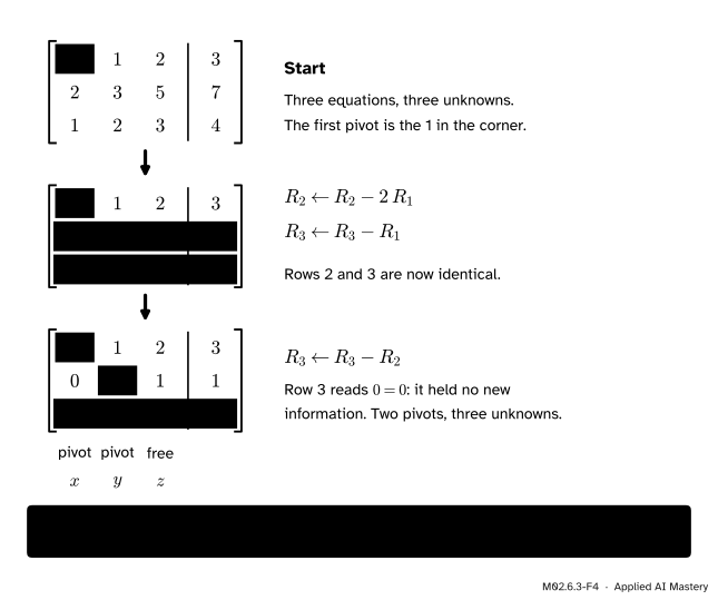
Elimination on a system whose third equation turns out to add nothing. Two pivots are left for three unknowns, so \(z\) is free.
Eliminate. The first pivot is the 1 in the corner. \({R_2 \leftarrow R_2 - 2R_1}\) gives \({(2 - 2,\; 3 - 2,\; 5 - 4 \mid 7 - 6)} = {(0,\; 1,\; 1 \mid 1)}\). \({R_3 \leftarrow R_3 - R_1}\) gives \({(1 - 1,\; 2 - 1,\; 3 - 2 \mid 4 - 3)} = {(0,\; 1,\; 1 \mid 1)}\). The second pivot is the 1 in row 2, and \({R_3 \leftarrow R_3 - R_2}\) gives \({(0,\; 0,\; 0 \mid 0)}\).
Classify. No row reads \(0 = c\) with \(c \neq 0\). Columns 1 and 2 are pivot columns. Column 3 has no pivot, so \(z\) is free. This is case 3.
Solve. Let \(z = t\). Row 2 says \(y + z = 1\), so \(y = 1 - t\). Row 1 says \(x + y + 2z = 3\), so \(x + {(1 - t)} + 2t = 3\), which gives \(x = 2 - t\). The general solution is
Check. With \(t = 0\), the point \((2, 1, 0)\) gives \(2 + 1 + 0 = 3\), then \(4 + 3 + 0 = 7\), then \(2 + 2 + 0 = 4\). With \(t = 1\), the point \((1, 0, 1)\) gives \(1 + 0 + 2 = 3\), then \(2 + 0 + 5 = 7\), then \(1 + 0 + 3 = 4\). The direction \((-1, -1, 1)\) gives \(-1 - 1 + 2 = 0\), then \(-2 - 3 + 5 = 0\), then \(-1 - 2 + 3 = 0\): it solves the system with zeros on the right, as the proof said it must.
In the row picture the three planes share a whole line, like three pages of a book meeting along the spine.
Change one number. Replace the last right-hand side, 4, by 5. The left-hand sides go through the same three operations. The right-hand side of row 3 becomes \(5 - 3 = 2\) and then \(2 - 1 = 1\), so the last row is \({[\,0 \;\; 0 \;\; 0 \mid 1\,]}\): case 1, no solution. Each pair of planes still meets in a line, but the three lines are parallel and no point lies on all three planes.
Code
From scratch: forward elimination that moves on when a column has no pivot, and a function that reads off the case.
import numpy as npdef echelon(A, b):"""Forward elimination that copes with missing pivots. Returns the echelon form and the pivot columns.""" M = np.column_stack([A, b]).astype(float) rows, n = M.shape[0], M.shape[1] -1 pivot_columns, r = [], 0for col inrange(n):if r == rows:break usable = [i for i inrange(r, rows) ifabs(M[i, col]) >1e-12]ifnot usable:continue# nothing to pivot on: this unknown is free M[[r, usable[0]]] = M[[usable[0], r]] # a swap, if one is neededfor i inrange(r +1, rows): M[i] = M[i] - (M[i, col] / M[r, col]) * M[r] pivot_columns.append(col) r +=1return M, pivot_columnsdef classify(A, b): M, pivot_columns = echelon(A, b) n = M.shape[1] -1for row in M:if np.allclose(row[:n], 0) andabs(row[n]) >1e-12:return"no solution"# a row that says 0 = c with c not zeroreturn"one solution"iflen(pivot_columns) == n else"infinitely many"row1 = [1, 1]print("lines cross: ", classify([row1, [-1, 2]], [3, 0]))print("lines parallel: ", classify([row1, [-1, -1]], [3, 0]))print("the same line: ", classify([row1, [-1, -1]], [3, -3]))S = np.array([[1, 1, 2], [2, 3, 5], [1, 2, 3]])M, pivot_columns = echelon(S, [3, 7, 4])print(M)print("pivot columns:", pivot_columns, "->", classify(S, [3, 7, 4]))print("with 5 in place of 4:", classify(S, [3, 7, 5]))
lines cross:     one solution
lines parallel:  no solution
the same line:   infinitely many
[[1. 1. 2. 3.]
 [0. 1. 1. 1.]
 [0. 0. 0. 0.]]
pivot columns: [0, 1] -> infinitely many
with 5 in place of 4: no solution
The pivot columns are numbered from 0 in code, so [0, 1] means the columns of \(x\) and \(y\). Now test the general solution for several values of \(t\).
particular = np.array([2, 1, 0])direction = np.array([-1, -1, 1])for t in (-2, 0, 0.5, 3):print(f"t = {t:>4}: S @ x =", S @ (particular + t * direction))print("S @ direction =", S @ direction)
t =   -2:  S @ x = [3 7 4]
t =    0:  S @ x = [3 7 4]
t =  0.5:  S @ x = [3. 7. 4.]
t =    3:  S @ x = [3 7 4]
S @ direction = [0 0 0]
The library version. NumPy counts pivots under the name rank, which lesson M02.7.2 studies. If attaching \(\vect{b}\) to the matrix raises the count, the extra pivot is in the last column, and that is the row \(0 = c\).
def pivots(M):returnint(np.linalg.matrix_rank(M))print("pivots of S:", pivots(S))print("with b = (3, 7, 4) attached:", pivots(np.column_stack([S, [3, 7, 4]])))print("with b = (3, 7, 5) attached:", pivots(np.column_stack([S, [3, 7, 5]])))try: np.linalg.solve(S, np.array([3.0, 7.0, 4.0]))except np.linalg.LinAlgError as error:print("numpy.linalg.solve:", error)
pivots of S: 2
with b = (3, 7, 4) attached: 2
with b = (3, 7, 5) attached: 3
numpy.linalg.solve: Singular matrix
numpy.linalg.solve is built for case 2 only. It refuses this matrix even when solutions exist, because there is no single answer to return.
Explore
The elimination stepper in lesson M02.6.2 has a preset for each case. Press Parallel lines or The same line and step once to see the rows \(0 = 3\) and \(0 = 0\) of this lesson’s first figure appear. Then try No common point and A shared line, which are the two versions of the worked example, and turn the view to see the three planes.
Pitfalls
M02.6.3-F5
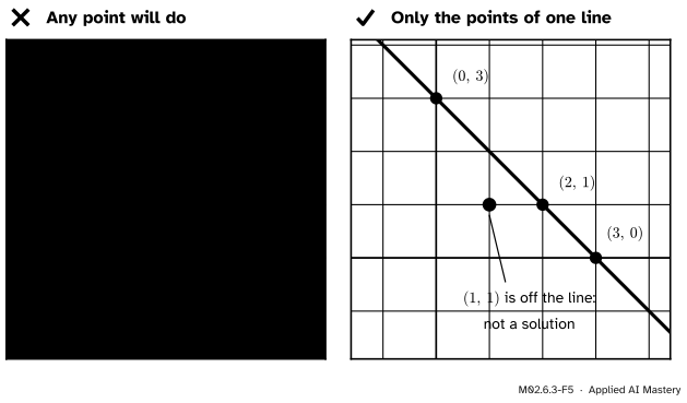
Wrong beside right. Infinitely many solutions is not the same as “everything is a solution”. The solutions fill one line, and a point off that line fails.
“Infinitely many solutions means any values will work.”
The solutions are the points \((3, 0) + t\,(-1, 1)\) and nothing else. The point \((1, 1)\) fails, because \(1 + 1 = 2\). A free variable is free, but once it is chosen the pivot variables are forced.
“A row of zeros means there is no solution.”
Look at the entry after the bar. The row \({[\,0 \;\; 0 \mid 0\,]}\) says \(0 = 0\), which is always true and removes nothing. The row \({[\,0 \;\; 0 \mid 3\,]}\) says \(0 = 3\), which is never true. Only the second kind means no solution.
“Three equations and three unknowns, so exactly one solution.”
Count pivots, not equations. The worked example has three equations and only two pivots, because one equation repeats what the others say. In machine learning this happens when one feature is a combination of others: the equations for the best weights lose a pivot, and infinitely many weight vectors fit equally well.
“More unknowns than equations cannot be solved.”
It cannot have exactly one solution, since there are at most as many pivots as rows and so some unknown is free. It has none or infinitely many. A linear model with more weights than training examples is in this position: if it can fit the data exactly at all, it can do so in infinitely many ways. Which of those fits a training method ends up with then matters a great deal, and it is an active topic of research.
Check yourself
Recall
1. What are the three possible numbers of solutions of a linear system?
Show answer
None, exactly one, or infinitely many.
2. After elimination, which kind of row shows that there is no solution?
Show answer
A row with zeros before the bar and a non-zero number after it. It says \(0 = c\) with \(c \neq 0\).
3. What is a free variable?
Show answer
An unknown whose column has no pivot in the echelon form. It can be given any value.
4. What does the row \({[\,0 \;\; 0 \;\; 0 \mid 0\,]}\) tell you?
Show answer
Nothing. It says \(0 = 0\). The equation it came from repeated information that the other equations already held.
5. If \(\vect{x}_1\) and \(\vect{x}_2\) both solve \(\mat{A}\vect{x} = \vect{b}\), what does \(\mat{A}\) do to \(\vect{x}_2 - \vect{x}_1\)?
Show answer
It sends it to zero: \(\mat{A}{(\vect{x}_2 - \vect{x}_1)} = \vect{b} - \vect{b} = \vect{0}\).
Exercises
1.★ Decide, by elimination, how many solutions each system has. (a) \(x + 2y = 4\) and \(2x + 4y = 8\). (b) \(x + 2y = 4\) and \(2x + 4y = 9\). (c) \(x + 2y = 4\) and \(2x + 5y = 9\).
Show solution
Apply \({R_2 \leftarrow R_2 - 2R_1}\) to each.
(a) The second row becomes \({(0,\; 0 \mid 0)}\): infinitely many solutions. With \(y = t\) they are \({(4 - 2t,\; t)}\).
(b) The second row becomes \({(0,\; 0 \mid 1)}\), which says \(0 = 1\): no solution.
(c) The second row becomes \({(0,\; 1 \mid 1)}\), so \(y = 1\) and \(x = 4 - 2 = 2\): one solution, \((2, 1)\).
2.★★ Find the general solution of the two equations \(x + 2y + z = 4\) and \(2x + 4y + 3z = 9\) in three unknowns. Which variable is free?
Show solution
\({R_2 \leftarrow R_2 - 2R_1}\) gives the row \({(0,\; 0,\; 1 \mid 1)}\). The echelon form is
The pivots are in columns 1 and 3, so the free variable is \(y\), the middle one. Let \(y = t\). Row 2 gives \(z = 1\). Row 1 gives \(x + 2t + 1 = 4\), so \(x = 3 - 2t\). The general solution is
Check with \(t = 1\): the point \((1, 1, 1)\) gives \(1 + 2 + 1 = 4\) and \(2 + 4 + 3 = 9\).
3.★★★ For which values of \(k\) and \(c\) does the system \(x + 2y = 1\), \(3x + ky = c\) have no solution, exactly one, or infinitely many?
Show solution
\({R_2 \leftarrow R_2 - 3R_1}\) gives the row \({(0,\; k - 6 \mid c - 3)}\).
If \(k \neq 6\), the entry \(k - 6\) is a pivot. There is exactly one solution, whatever \(c\) is: \(y = {(c - 3)}/{(k - 6)}\) and \(x = 1 - 2y\).
If \(k = 6\) and \(c = 3\), the row is \({(0,\; 0 \mid 0)}\). There are infinitely many solutions, \({(1 - 2t,\; t)}\).
If \(k = 6\) and \(c \neq 3\), the row says \(0 = c - 3\) with \(c - 3 \neq 0\). There is no solution.
The matrix alone (\(k\)) decides between “exactly one” and “none or infinitely many”. The right-hand side (\(c\)) then decides between none and infinitely many.
Summary card
Eliminate, then read the last rows: none, one, or infinitely many.
M02.6.3-F1
A pivot, a contradiction, or nothing.
No solution. Some row reads \(0 = c\) with \(c \neq 0\).
One solution. No such row, and every column has a pivot.
Infinitely many. No such row, and at least one free variable.
General solution. One particular solution plus all solutions of \(\mat{A}\vect{x} = \vect{0}\).
Never two.\(\mat{A}{\big(\vect{x}_1 + t(\vect{x}_2 - \vect{x}_1)\big)} = \vect{b}\) for every \(t\).
Sources and next steps
Sources. Each was opened and checked against this lesson on 12 November 2026.
Dan Margalit and Joseph Rabinoff, Interactive Linear Algebra, Georgia Institute of Technology (open access). Section 1.1 draws the three cases for two lines (one point, parallel lines, the same line) and defines consistent and inconsistent systems. Section 1.3 defines a free variable as one whose column is not a pivot column and lists the three possibilities by pivots: the last column is a pivot column (no solutions), every other column is a pivot column (a unique solution), or neither (infinitely many).
Gilbert Strang, Solving Ax = b: row reduced form R, MIT OpenCourseWare 18.06SC, with its lecture summary. It tests solvability by elimination on the augmented matrix, finds a particular solution by setting the free variables to zero, builds the complete solution from it, and ends with a table in which the number of solutions is always 0, 1 or infinitely many.
Next.M02.6.4 Elimination as matrices shows that every row operation is a matrix multiplication, which is how libraries organise the work.