A matrix whose rows are probabilities moves a distribution forward one step at a time. Build the transition matrix of a chain, prove that 1 is always an eigenvalue and that no eigenvalue is larger, and find the long run of a two-state chain by diagonalising.
M03.9.1L2 Intermediate25 minIn review (what this means)
The maths and code on this page are checked by automated tests on every change, but an independent reader has not signed it off yet. Spot a mistake or a confusing step? Tell us.
Write the row-stochastic transition matrix of a chain from its state diagram, and its transpose in the column convention.
Move a distribution one step forward with the update pi_(t+1) = P-transpose pi_t, derived from the law of total probability.
Prove that every Markov matrix has the eigenvalue 1 and that no eigenvalue exceeds 1 in modulus.
Find the stationary distribution and the distribution at every step of a two-state chain by diagonalising.
The question
If today is dry, tomorrow is dry with probability 0.9; if today is wet, tomorrow is wet with probability 0.5. Start on a dry day. What is the chance that the day a month from now is dry, and why does the answer stop depending on where you started?
Intuition
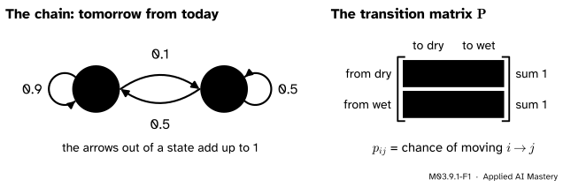
A Markov chain hops between a few states. Where it goes next depends only on where it is now, through fixed probabilities. Draw each state as a circle and each possible move as an arrow labelled with its probability: that is a state diagram.
Then write the same numbers in a table, one row for each state of today and one column for each state of tomorrow. That table is the transition matrix\(\mat{P}\).
M03.9.1-F1
The running chain of the course. Row \(i\) of \(\mat{P}\) lists the arrows that leave state \(i\), so every row adds up to 1: tomorrow has to be something.
The matrix holds the whole chain. The question is what it does to probabilities when it is applied again and again, and the answer is in its eigenvalues.
Build it up
Step 1. A distribution is a vector. Write \(\vect{\pi}_t\) for the chances of each state on day \(t\), as a column. A dry start is \(\vect{\pi}_0 = (1, 0)\). Its entries are at least 0 and add up to 1: it is a probability vector, or distribution.
Step 2. One day forward, by the law of total probability. Tomorrow is dry if today is dry and the chain stays, or today is wet and the chain moves (M06.3):
The numbers \(0.9\) and \(0.5\) are the first column of \(\mat{P}\). In general entry \(j\) of tomorrow is \({\sum_i \pi_t(i)\,p_{ij}}\), which is entry \(j\) of \(\mat{P}\T\vect{\pi}_t\). So
\[
\vect{\pi}_{t+1} = \mat{P}\T\vect{\pi}_t .
\]
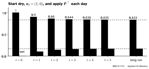
Step 3. Day by day. From the dry start, \(\vect{\pi}_1 = (0.9, 0.1)\), the first row of \(\mat{P}\). Then \(\vect{\pi}_2 = {(0.81 + 0.05,\; 0.09 + 0.05)} = (0.86, 0.14)\), and so on.
M03.9.1-F2
The distribution of the running chain from a dry start. The dry bar falls towards \(5/6 \approx
0.833\) and the wet bar rises towards \(1/6\), closing most of the remaining gap every day.
Step 4. Two conventions, one chain. Strang’s lectures and Austin’s textbook write the same chain with columns that add to 1. Their matrix is our \(\mat{P}\T\), and their update multiplies the distribution by that matrix directly. This course keeps rows that add to 1, as in reinforcement learning (\(\mat{P}_\pi\) in NOTATION) and in the probability course M07.7, and pays for it with the transpose in the update.
The formal statement
NoteDefinition: Markov matrix
An \(n \times n\) matrix \(\mat{P}\) is a Markov matrix (or row-stochastic) when every entry is at least 0 and every row adds up to 1. Entry \(p_{ij}\) is the probability of moving from state \(i\) to state \(j\). A distribution \(\vect{\pi}\) with \(\mat{P}\T\vect{\pi} = \vect{\pi}\) is a stationary distribution, or steady state.
Distributions stay distributions. Write \(\vect{1}\) for the vector of ones. “Every row adds up to 1” says exactly \(\mat{P}\vect{1} = \vect{1}\). The entries of \(\mat{P}\T\vect{\pi}\) are sums of products of non-negative numbers, so they are non-negative. Their total is
The number 1 is an eigenvalue of \(\mat{P}\) and of \(\mat{P}\T\).
Every eigenvalue \(\lambda\), real or complex, has \(\abs{\lambda} \le 1\).
Proof of 1.\(\mat{P}\vect{1} = \vect{1}\) says that \(\vect{1}\) is an eigenvector of \(\mat{P}\) for the eigenvalue 1. A matrix and its transpose have the same eigenvalues, because a determinant does not change under transposing (M02.8):
So 1 is an eigenvalue of \(\mat{P}\T\) too. Its eigenvector is a steady state, but it is not\(\vect{1}\): the two matrices share eigenvalues, not eigenvectors (exercise 3 of M03.1.2).
Proof of 2. Let \(\mat{P}\vect{v} = \lambda\vect{v}\) with \(\vect{v} \ne \vect{0}\), and pick an index \(i\) where \(\abs{v_i}\) is largest. Row \(i\) of the equation is \(\lambda v_i = {\sum_j p_{ij} v_j}\). Take sizes and use the triangle inequality:
The second line uses \({\abs{v_j} \le \abs{v_i}}\) and that row \(i\) adds to 1. Divide by \({\abs{v_i} > 0}\) to get \(\abs{\lambda} \le 1\). The same lines work for complex \(\lambda\) and \(\vect{v}\). In the language of M03.8.1, the max-norm of \(\mat{P}\) is its largest row sum, 1, and no eigenvalue can exceed a norm. The eigenvalues of \(\mat{P}\T\) are the same numbers, so they obey the same bound. \(\blacksquare\)
M03.9.1-F3
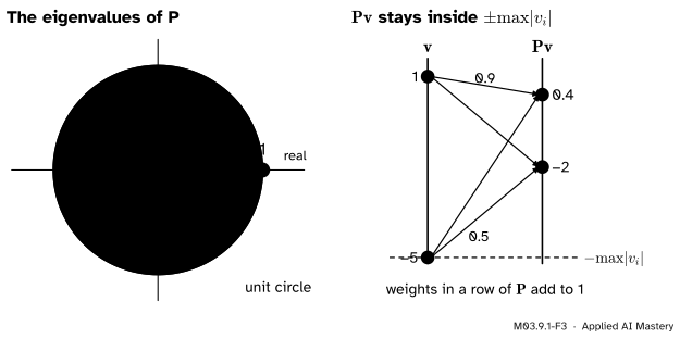
Why no eigenvalue is bigger than 1. Each entry of \(\mat{P}\vect{v}\) is a weighted average of the entries of \(\vect{v}\), so it cannot be larger in size than the largest of them. Here \(\vect{v} = (1, -5)\) and \(\mat{P}\vect{v} = (0.4, -2) = 0.4\,\vect{v}\).
Worked example
Find the eigenvalues of the running chain, its stationary distribution, and the distribution on every day from a dry start.
Eigenvalues.\(\mat{P}\T\) has rows \((0.9, 0.5)\) and \((0.1, 0.5)\), trace \(1.4\) and determinant \({0.45 - 0.05} = 0.4\). Its characteristic polynomial (M03.1.2) is
Steady state. For \(\lambda = 1\) the first row of \(\mat{P}\T - \mat{I}\) is \((-0.1, 0.5)\), so \({-0.1x + 0.5y} = 0\), that is, \(x = 5y\). The eigenvector \((5, 1)\), divided by its sum 6, is the distribution \(\vect{\pi} = (5/6, 1/6)\).
The other eigenvector. For \(\lambda = 0.4\) the first row of \(\mat{P}\T - 0.4\mat{I}\) is \((0.5, 0.5)\), so \({x + y} = 0\) and the eigenvector is \((1, -1)\). Its entries add to 0, so adding any multiple of it to a distribution keeps the total at 1.
Every day at once. Write the start in the eigenvector basis, \(\vect{\pi}_0 =
{\vect{\pi} + c\,(1, -1)}\). Comparing first entries, \(1 = 5/6 + c\), so \(c = 1/6\). Applying \(\mat{P}\T\) multiplies the first part by 1 and the second by 0.4 (M03.2.2), so
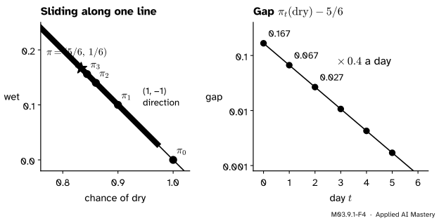
The running chain from a dry start. Every distribution lies on the line where the chances add to 1, and the chain slides along the eigenvector direction \((1, -1)\) towards the steady state. The gap is multiplied by the second eigenvalue, 0.4, every day.
A month is about 30 days, and \(\tfrac16(0.4)^{30} \approx 2 \times 10^{-13}\). So the chance of a dry day a month from now is \(5/6\) to twelve decimal places, wherever the chain started. That answers the hook. A wet start has \(c = -5/6\) and reaches the same place.
Code
From scratch: step the distribution forward and compare with the formula.
import numpy as npP = np.array([[0.9, 0.1], [0.5, 0.5]])assert np.allclose(P.sum(axis=1), 1) # rows add to 1pi = np.array([1.0, 0.0]) # a dry starthistory = [pi]for day inrange(30): pi = P.T @ pi # one day forward history.append(pi)history = np.array(history)print(history[:4])print("day 30:", history[30])
Now the library. The steady state is the eigenvector of \(\mat{P}\T\) for the eigenvalue 1. numpy.linalg.eig returns its columns scaled to length 1, with any sign, so divide by the sum to turn the column into a distribution.
w, V = np.linalg.eig(P.T)k = np.argmin(np.abs(w -1)) # the eigenvalue closest to 1stationary = V[:, k] / V[:, k].sum() # rescale to add to 1print("eigenvalues:", w)print("column from eig:", V[:, k], "-> distribution:", stationary)print("P to the power 30:\n", np.linalg.matrix_power(P, 30))
eigenvalues: [1. +0.j 0.4+0.j]
column from eig: [0.98058068+0.j 0.19611614+0.j] -> distribution: [0.83333333+0.j 0.16666667+0.j]
P to the power 30:
 [[0.83333333 0.16666667]
 [0.83333333 0.16666667]]
The last print shows something worth stopping for: every row of \(\mat{P}^{30}\) is \((5/6, 1/6)\). Row \(i\) of \(\mat{P}^t\) holds the chances of being in each state \(t\) days after starting in state \(i\), so the rows becoming equal is the chain forgetting its start.
Explore
This module’s interactive, the random surfer, lives in lesson M03.9.4. It runs the same update \({\vect{\pi}_{t+1} = \mat{P}\T\vect{\pi}_t}\) on a chain with four states, one click at a time, and prints the distance from the steady state after every step.
Pitfalls
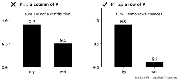
M03.9.1-F5
Wrong beside right, from the dry start \(\pi_0 = (1, 0)\). Multiplying by \(\mat{P}\) picks out a column, which mixes the chances of arriving from different states. Multiplying by \(\mat{P}\T\) picks out the row of the current state.
“The next distribution is \(\mat{P}\vect{\pi}_t\).”
Not with rows that add to 1. The product \(\mat{P}\vect{\pi}_0\) for \(\vect{\pi}_0 = (1, 0)\) is the first column, \((0.9, 0.5)\), whose entries add to 1.4. The quick test: after one step the entries must still add to 1. If you write distributions as rows instead, the update is \({\vect{\pi}_{t+1}\T = \vect{\pi}_t\T\mat{P}}\), which is the same equation transposed.
“The steady state is the eigenvector of \(\mat{P}\) for the eigenvalue 1.”
For every Markov matrix one such eigenvector is \(\vect{1}\), here \((1, 1)\), and it carries no information about the chain. The steady state is the eigenvector of \(\mat{P}\T\) for the eigenvalue 1, here \((5, 1)\) up to scale. The eigenvalue is shared, the eigenvector is not.
“The column that eig returns is the steady state.”
It points the right way but has length 1 and may come out negative: here about \(\pm(0.981, 0.196)\). Divide by its sum, not by its length, to get \((5/6, 1/6)\). In machine learning the same slip turns a vector of class weights or of page ranks into numbers that do not add to 1.
Check yourself
Recall
1. What do the rows of a Markov matrix add up to, and what does entry \(p_{ij}\) mean?
Show answer
Each row adds up to 1. Entry \(p_{ij}\) is the probability of moving from state \(i\) to state \(j\) in one step.
2. How does a distribution move one step forward in the row convention?
Show answer
\(\vect{\pi}_{t+1} = \mat{P}\T\vect{\pi}_t\), from the law of total probability: entry \(j\) is \(\sum_i \pi_t(i)\,p_{ij}\).
3. Why is 1 always an eigenvalue of \(\mat{P}\T\)?
Show answer
\(\mat{P}\vect{1} = \vect{1}\) because the rows add to 1, so 1 is an eigenvalue of \(\mat{P}\); and \(\mat{P}\) and \(\mat{P}\T\) have the same characteristic polynomial, hence the same eigenvalues.
4. What is the stationary distribution of the running chain, and its other eigenvalue?
Show answer
\(\vect{\pi} = (5/6, 1/6)\), and the other eigenvalue is \(0.4\), with eigenvector \((1, -1)\).
5. In the column convention of Strang and Austin, what is their matrix in terms of ours?
Show answer
Their matrix is \(\mat{P}\T\): its columns add to 1, and their update, which multiplies by that matrix directly, is our \(\vect{\pi}_{t+1} = \mat{P}\T\vect{\pi}_t\).
Exercises
1.★ Start the running chain on a wet day, \(\vect{\pi}_0 = (0, 1)\). Find \(\vect{\pi}_1\) and \(\vect{\pi}_2\) by multiplying, and check them against the formula with \(c = -5/6\).
Show solution
\(\vect{\pi}_1 = \mat{P}\T(0, 1) = (0.5, 0.5)\), the second row of \(\mat{P}\). Then
The formula gives \(\pi_t(\text{dry}) = {5/6 - (5/6)(0.4)^t}\): for \(t = 1\), \({5/6 - 1/3} = 0.5\), and for \(t = 2\), \({5/6 - 0.8/6} = {4.2/6} = 0.7\). They match.
2.★★ A general two-state chain has \(\mat{P} = \begin{bmatrix} 1 - a & a \\ b & 1 - b \end{bmatrix}\) with \(0 < a, b \le 1\). Find its stationary distribution and its second eigenvalue, and check them on the running chain.
Show solution
The trace of \(\mat{P}\T\) is \({2 - a - b}\) and the eigenvalues are 1 and the second eigenvalue \(\lambda_2\), which add up to the trace, so \({\lambda_2 = 1 - a - b}\). For the steady state, the first row of \(\mat{P}\T - \mat{I}\) is \((-a, b)\), so \({-a x + b y} = 0\) and \((x, y)\) is a multiple of \((b, a)\). Dividing by the sum,
The running chain has \(a = 0.1\) and \(b = 0.5\): \(\vect{\pi} = (0.5/0.6,\; 0.1/0.6) = (5/6, 1/6)\) and \({\lambda_2 = 1 - 0.6} = 0.4\).
3.★★★ Show that the product of two Markov matrices of the same size is a Markov matrix. Deduce that every power \(\mat{P}^t\) is one, and explain in words what its row \(i\) means.
Show solution
Let \(\mat{P}\) and \(\mat{Q}\) be Markov. Every entry of \(\mat{P}\mat{Q}\) is a sum of products of non-negative numbers, so it is non-negative. For the row sums, \({(\mat{P}\mat{Q})\vect{1} = \mat{P}(\mat{Q}\vect{1})} = {\mat{P}\vect{1}} = \vect{1}\). So \(\mat{P}\mat{Q}\) is Markov. By induction on \(t\), with \(\mat{P}^{t+1} = \mat{P}^t\mat{P}\), every power is Markov. Row \(i\) of \(\mat{P}^t\) is \((\mat{P}\T)^t\) applied to the start \(\vect{e}_i\), written as a row: the distribution \(t\) steps after starting in state \(i\), which is why its entries add up to 1.
Summary card
Rows of probabilities move a distribution forward, and the eigenvalue 1 holds the long run.
M03.9.1-F1
One row per state of today.
Markov matrix.\(p_{ij} \ge 0\) and every row adds to 1: \(\mat{P}\vect{1} = \vect{1}\).
Sources. Each was opened and checked against this lesson on 15 November 2026.
Gilbert Strang, Markov matrices; Fourier series, MIT OpenCourseWare 18.06SC, lecture 24 and its summary. Markov matrices with columns adding to 1 (the transpose of ours), the argument that the columns of \(A - I\) adding to zero make it singular so that 1 is an eigenvalue, the fact that \(A\) and \(A\T\) share eigenvalues, and a two-state migration example.
Dan Margalit and Joseph Rabinoff, Interactive Linear Algebra, section 5.6 Stochastic matrices (Georgia Tech). A stochastic matrix has non-negative entries and columns adding to 1; the Fact that 1 is an eigenvalue and every real or complex eigenvalue has \(\abs{\lambda} \le 1\), with proof.
NumPy reference, numpy.linalg.eig: eigenvalues in no particular order, eigenvectors as unit-length columns.
Next.M03.9.2 Steady states and Perron-Frobenius asks when the steady state is unique and always reached, and what goes wrong when it is not. Chains as models of random processes, with hitting times and recurrence, are the subject of M07.7, and the transition matrix \(\mat{P}_\pi\) of a policy drives the Bellman equations of RL01.