k-means looks for round clusters of similar spread and size, because J measures squared distance to a single centre. See each failure beside the right answer, with stretched blobs, moons, unequal spreads, mixed units and an outlier, and meet k-medoids and its PAM swap step.
ML03.1.4L2 Intermediate25 minIn review (what this means)
The maths and code on this page are checked by automated tests on every change, but an independent reader has not signed it off yet. Spot a mistake or a confusing step? Tell us.
Explain, from the straight borders between Voronoi cells, why k-means favours round clusters of similar spread and size.
Recognise stretched, unequal, non-convex and badly scaled data on which the lowest J is the wrong answer.
Show how standardising the features changes a k-means clustering.
Compute k-medoids by hand with the PAM swap step and explain why it resists an outlier.
Name the method of this course that repairs each failure.
The question
k-means always returns \(K\) clusters, and the last lesson showed how to make sure they have the lowest \(J\) it can find. But is “lowest \(J\)” the same as “the groups that are really in the data”? When is the best answer to k-means’ question the wrong answer to ours?
From the last lesson
1. How does k-means++ choose each new centre?
Show answer
With probability proportional to \(D(\vect{x})^2\), the squared distance from a point to the nearest centre already chosen.
2. On a plot of \(J\) against \(K\), what should you look for?
Show answer
A bend (an elbow), where the big drops stop. Not the minimum, which is always at the largest \(K\).
Intuition
k-means has one idea of a cluster: a cloud of points around a centre, judged by squared distance, the same in every direction. Its regions are Voronoi cells, and the border between two cells is the straight line halfway between their centres. Data that look like that are clustered well. Data that do not are cut wherever the straight lines fall.
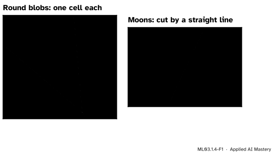
ML03.1.4-F1
k-means draws straight borders halfway between centres. Round, similar blobs fall one to a cell. Two interlocking moons cannot: a straight line cuts each of them in two.
Each failure below has the same cause. Look for it in every picture: the borders depend only on where the centres are, never on the shape, spread or size of the clusters.
Build it up
The data are scikit-learn’s own demonstration of the k-means assumptions, plus three small sets of our own. In each figure the true groups are shown by shape and colour, the tints are k-means’ cells, and points that land in the wrong cluster are ringed in reddish purple.
Step 1. Stretched clusters. Take three round blobs and shear the plane, so that each becomes a long thin ellipse. The ellipses lie side by side, closer across than along.
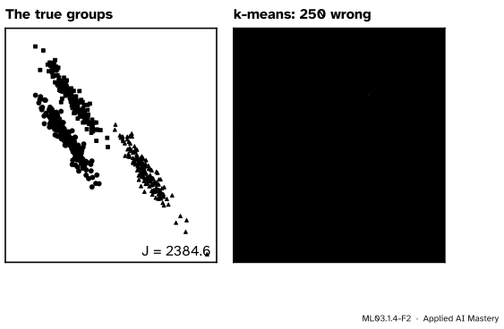
ML03.1.4-F2
Stretched clusters. The k-means answer cuts across the ellipses and puts 250 of the 1500 points in the wrong group, yet its \(J = 1899.3\) is lower than the true grouping’s \(J = 2384.6\).
k-means has not failed at its own task. It found a lower \(J\) than the truth. The objective itself is the problem: it rewards round clusters, so cutting an ellipse across its width wins.
Step 2. Unequal spreads, unequal sizes. Now give the clusters different spreads, or very different numbers of points.
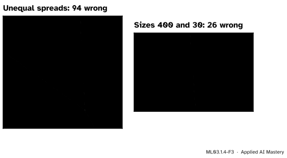
ML03.1.4-F3
Left: a wide cluster beside tight ones loses 94 points to them. Right: a cluster of 400 points beside one of 30, with the same spread, loses 26 points to it.
Both failures come from the border. It sits halfway between the centres whatever the clusters look like, so a wide cluster cannot claim the extra room its spread needs. For sizes, the small cluster’s centre is pulled towards the big cluster’s edge points that it takes over, and the border follows.
Step 3. Shapes that are not convex. Every Voronoi cell is convex: a polygon with no dents. The moons are not, and no arrangement of two convex cells can hold them. k-means with \(K = 2\) puts 76 of the 300 moon points in the wrong group.
Step 4. Units and outliers. Two more failures do not depend on shape at all: a feature measured in big numbers that drowns the others, and a single far point that drags a centre. The pitfalls and the worked example take them in turn.
The formal statement
Why k-means wants round, equal clusters. Three facts from the first two lessons explain every failure above.
First,\(J\) adds squared Euclidean distances to one centre, and a distance counts the same in every direction. A long, thin cluster pays for its whole length, so cutting it across its length and handing the pieces to nearby centres can lower \(J\), as in Step 1. What \(J\) rewards is clusters that are compact in every direction: round ones.
Second, the border between the cells of \(\vect{\mu}_1\) and \(\vect{\mu}_2\) is the set of \(\vect{x}\) with
which involves the centres and nothing else: not the clusters’ spreads, not their sizes.
Third, every cell is an intersection of half-planes, so it is convex.
scikit-learn’s demonstration puts the same point in statistical terms: k-means behaves like a mixture of Gaussians that all have the same, round spread. Lesson ML03.4 lets each Gaussian have its own shape, size and weight.
NoteDefinition: k-medoids
Choose \(K\)medoids\(\vect{m}_1, \dots, \vect{m}_K\)from the data points themselves, and any dissimilarity \(d\) (it need not be a squared distance, or even a metric). Each point joins its nearest medoid, and the objective is the total deviation
With \(d\) the plain distance, one far point adds its distance, not its squared distance, and a medoid can never sit out in empty space, because it must be a data point.
PAM (Partitioning Around Medoids). Kaufman and Rousseeuw’s algorithm has two phases. BUILD chooses \(K\) starting medoids greedily, each time adding the point that lowers \(\mathit{TD}\) most. SWAP then improves them:
For every medoid \(\vect{m}\) and every non-medoid \(\vect{o}\), compute \(\mathit{TD}\) with \(\vect{o}\) in place of \(\vect{m}\). There are \(K(n - K)\) such swaps.
If the best swap lowers \(\mathit{TD}\), make it and go back to step 1. Otherwise stop.
Like Lloyd’s algorithm, each step lowers the objective, so PAM stops at a local optimum. It is slower: done naively each swap needs a pass over all \(n\) points, and Schubert and Rousseeuw give the cost of one round of SWAP as \(O(K (n - K)^2)\) even with cached distances.
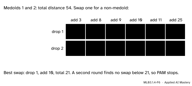
ML03.1.4-F6
One round of PAM’s SWAP on the line values, from the medoids \(1\) and \(2\). All \(2 \times 6 = 12\) swaps are scored; the best, \(1 \to 10\), lowers \(\mathit{TD}\) from \(54\) to \(21\).
Worked example
Eight values on a line, \(1, 2, 3\) and \(8, 9, 10, 11\), plus one outlier at \(25\). Cluster them with \(K = 2\).
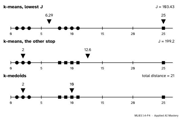
The grouping we want.\(\{1, 2, 3\}\) and \(\{8, 9, 10, 11, 25\}\). The second mean is \({63/5} = 12.6\), beyond every point of the group: the outlier has dragged it. Within the first group, \(J\) is \(1 + 0 + 1 = 2\). In the second it is
so \(J = 199.2\). Lloyd’s algorithm can stop here: the border is at \({(2 + 12.6)/2} = 7.3\), so every point is in its own cell.
k-means’ best answer. On a line the best clusters are runs of neighbours, so only seven splits need checking. The lowest \(J\) puts \(25\) alone and the other seven together, with mean \({44/7} \approx 6.286\):
So k-means’ best answer spends a whole cluster on one outlier and merges the two real groups.
k-medoids with plain distance. With medoids \(2\) and \(10\), the distances are \(1, 0, 1\) and \(2, 1, 0, 1, 15\), so \(\mathit{TD} = 21\). Giving \(25\) its own medoid instead, the other seven are best served by \(8\), with distances \(7, 6, 5, 0, 1, 2, 3\) that add to \(24\). Since \(24 > 21\), the medoids keep the real groups, and each sits on a real point.
ML03.1.4-F4
One outlier, three answers. k-means’ lowest \(J\) isolates the outlier (top). The grouping we want is only a local minimum of \(J\), with a centre dragged to \(12.6\) (middle). k-medoids keeps the groups and puts its centres on real points (bottom).
Code
First the failures, measured. A helper relabels the clusters to match the true groups as well as possible, then counts the points that disagree.
import itertoolsimport numpy as npfrom sklearn.cluster import KMeansfrom sklearn.datasets import make_blobs, make_moonsdef wrong(y, z):"""Points in the wrong group, after the best renumbering of the clusters.""" K =max(y.max(), z.max()) +1returnmin(int(np.sum(np.array(p)[z] != y)) for p in itertools.permutations(range(K)))def J_true(X, y):returnsum(((X[y == k] - X[y == k].mean(axis=0)) **2).sum() for k in np.unique(y))X, y = make_blobs(n_samples=1500, random_state=170) # scikit-learn's exampledata = {"stretched": (X @ np.array([[0.60834549, -0.63667341], [-0.40887718, 0.85253229]]), y, 3),"unequal spreads": (*make_blobs(n_samples=1500, cluster_std=[1.0, 2.5, 0.5], random_state=170), 3),"sizes 400 and 30": (*make_blobs(n_samples=[400, 30], centers=[(0, 0), (4.5, 0)], random_state=0), 2),"moons": (*make_moons(n_samples=300, noise=0.05, random_state=0), 2),}results = {}for name, (Xs, ys, K) in data.items(): km = KMeans(n_clusters=K, n_init=10, random_state=0).fit(Xs) results[name] = (wrong(ys, km.labels_), km.inertia_, J_true(Xs, ys))print(f"{name:17s} wrong {results[name][0]:4d} J k-means {km.inertia_:8.1f} J true {J_true(Xs, ys):8.1f}")
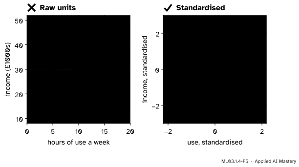
In every case k-means’ \(J\) is lower than the true grouping’s \(J\). Now the units. Hours of use a week separate two kinds of customer; income, in pounds, does not, but its numbers are thousands of times larger.
Gaussian mixture on stretched blobs: 0 wrong
DBSCAN on moons: 0 wrong;  noise points: 0
Explore
In the k-means stepper, load anisotropic blobs, unequal sizes and moons in turn and run Lloyd’s algorithm to the end, from several starts. The read-out compares the final \(J\) with the \(J\) of the groups the points were drawn from. Then load the nine points, drag one point far to the right, run Lloyd’s algorithm again, and watch a centre follow it.
Pitfalls
ML03.1.4-F5
Wrong beside right. In raw units income, measured in pounds, decides every distance, and k-means splits the customers by income: 57 of 120 wrong. After standardising, hours of use counts, and none are wrong.
“Distances are distances; the units do not matter.”
A difference of 8,000 pounds outweighs any difference in hours, so k-means sees only income. As in ML01.3.3, standardise each feature first (subtract its mean, divide by its standard deviation), inside a pipeline. But standardising gives every feature an equal say, including a feature that is pure noise, so it is a choice, not a cure.
“The k-means answer has the lower J, so it must be the better clustering.”
On every data set of this lesson, the true groups have a higher\(J\) than k-means’ answer. \(J\) is a score of roundness and tightness. When the real groups are not round and tight, the lowest \(J\) is the wrong answer, and no amount of restarting will fix it.
“k-means found three clusters, so the data contain three round groups.”
k-means returns \(K\) clusters for any data, even uniform noise. It never reports that the groups are stretched, curved or absent. Look at the data, and use the methods of ML03.10 to ask whether the structure is real.
Check yourself
Recall
1. Why are the borders of k-means’ clusters straight lines?
Show answer
The border between two centres is where the squared distances are equal, and the \(\norm{\vect{x}}^2\) terms cancel, leaving an equation that is linear in \(\vect{x}\).
2. Why can a wide cluster beside a tight one lose points to it?
Show answer
The border sits halfway between the centres whatever the spreads are, so the wide cluster’s far edge lands in its neighbour’s cell.
3. What two things does k-medoids change compared with k-means?
Show answer
Each centre must be one of the data points (a medoid), and any dissimilarity can be used, such as the plain distance instead of the squared distance.
4. What does one round of PAM’s SWAP step do?
Show answer
It scores every swap of a medoid with a non-medoid, \(K(n - K)\) of them, and makes the best one if it lowers the total deviation; otherwise PAM stops.
5. Which method of this course repairs stretched clusters, which repairs moons?
Show answer
Gaussian mixtures (ML03.4) for stretched clusters of different shapes and sizes; density-based clustering (ML03.3) or spectral clustering (ML03.6.1) for moons and other non-convex shapes.
Exercises
1.★ A cluster holds the values \(1, 2, 3, 4, 20\). Find its mean and its medoid under plain distance. Which one is a typical member of the cluster?
Show solution
The mean is \({30/5} = 6\), larger than four of the five values. For the medoid, add the distances from each candidate: \(1\) gives \({0 + 1 + 2 + 3 + 19} = 25\), \(2\) gives \(22\), \(3\) gives \(21\), \(4\) gives \(22\) and \(20\) gives \(70\). The medoid is \(3\), one of the two middle values of the four ordinary ones: the outlier barely moves it, while it drags the mean to \(6\).
2.★★ Two features: one is a length in metres with a standard deviation of \(0.1\), the other a mass in grams with a standard deviation of \(500\). Two points differ by one standard deviation in each feature. What share of their squared distance comes from the mass? What is it after standardising?
Show solution
The squared distance is \(0.1^2 + 500^2 = 0.01 + 250000\), so the mass gives \({250000 / 250000.01}\), more than \(99.99\) percent. After standardising, each difference is one unit, so the squared distance is \({1 + 1} = 2\) and each feature gives half.
3.★★★ Run one round of PAM’s SWAP by hand on the values \(0, 1, 2, 10, 11\) with \(K = 2\) and plain distance, starting from the medoids \(0\) and \(1\). Which swap is best, and does a second round improve on it?
Show solution
At the start, \(\mathit{TD} = 0 + 0 + 1 + 9 + 10 = 20\). The swaps that bring in \(10\) or \(11\) are the only useful ones. Replacing \(0\) by \(10\) (medoids \(1, 10\)): distances \(1, 0, 1, 0, 1\), so \(\mathit{TD} = 3\). Replacing \(0\) by \(11\): \(1, 0, 1, 1, 0\), so \(\mathit{TD} = 3\) too. Replacing \(1\) by \(10\) (medoids \(0, 10\)): \(0, 1, 2, 0, 1\), so \(\mathit{TD} = 4\); by \(11\): \(\mathit{TD} = 4\). Swaps that bring in \(2\) leave \(10\) and \(11\) at distance \(8\) or more from both medoids, so \(\mathit{TD} \ge 17\). The best swap lowers \(\mathit{TD}\) to \(3\); taking the first one found, PAM moves to medoids \(1\) and \(10\). In the second round, no swap does better: the medoid of \(\{0, 1, 2\}\) is \(1\) (cost \(2\)) and either \(10\) or \(11\) costs \(1\) for \(\{10, 11\}\), so \(\mathit{TD} = 3\) is the lowest possible. PAM stops.
Summary card
k-means finds round, similar, convex clusters, whatever the data hold.
Fails on. Stretched, unequally spread or sized, non-convex clusters; mixed units; outliers.
Lowest J is not truth. Every failure here has \(J\) below the true groups’ \(J\).
k-medoids. Centres are data points, any dissimilarity; PAM swaps a medoid for a point while \(\mathit{TD}\) falls.
Repairs. Mixtures (ML03.4), density (ML03.3), spectral (ML03.6.1).
Sources and next steps
Sources. Each was opened and checked against this lesson on 15 November 2026.
scikit-learn developers, Demonstration of k-means assumptions, version 1.9. The data of Steps 1 and 2: make_blobs with n_samples=1500 and random_state=170, the transformation matrix for the anisotropic blobs and cluster_std=[1.0, 2.5, 0.5]; the remarks that k-means is suited to isotropic clusters, behaves like a mixture of Gaussians with equal variances, and that a Gaussian mixture fixes the anisotropic and unequal-variance cases.
scikit-learn developers, User Guide, Section 2.3.2 K-means, version 1.9. Inertia assumes that clusters are convex and isotropic and responds poorly to elongated clusters or manifolds with irregular shapes.
Erich Schubert and Peter J. Rousseeuw, Faster k-Medoids Clustering: Improving the PAM, CLARA, and CLARANS Algorithms, SISAP 2019. Section 1 defines the total deviation \(\mathit{TD}\) and the medoid; Section 2 describes PAM’s BUILD and SWAP (Algorithms 1 and 2), the \(k(n - k)\) candidate swaps and the cost \(O(k(n - k)^2)\) per iteration.
Trevor Hastie, Robert Tibshirani and Jerome Friedman, The Elements of Statistical Learning, 2nd edition. Section 14.3.10, K-medoids: squared Euclidean distance gives the largest distances the most influence, so k-means lacks robustness against outliers; restricting each centre to an observation allows any dissimilarity, and makes the method far more computationally intensive (Algorithm 14.2).
Next. Each failure has its own repair later in this course: hierarchical clustering (ML03.2) builds clusters from merges instead of centres, density-based clustering (ML03.3) follows any shape, and Gaussian mixtures (ML03.4) give each cluster its own shape, spread and weight.