Write the first-order change df in terms of the change dX, rearrange it into tr(G-transpose dX), and read off the gradient G. Derive least squares, ridge and three matrix gradients this way, without a single index.
M05.7.2L2 Intermediate25 minIn review (what this means)
The maths and code on this page are checked by automated tests on every change, but an independent reader has not signed it off yet. Spot a mistake or a confusing step? Tell us.
Explain why df = tr(G-transpose dX) identifies G as the gradient with respect to the matrix X.
Apply the rules d(AXB) = A dX B, the product rule and the transpose rule, and use the cyclic property of the trace.
Derive the gradients of tr(AX), a-transpose X b, the squared Frobenius norm of AX - B, least squares and ridge regression with differentials.
Check a matrix gradient entry by entry against finite differences.
The question
Index notation works, but for \(\norm{\mat{A}\mat{X} - \mat{B}}_F^2\) it needs four letters and a lot of care. Worse, a guess is easy to get backwards: is the gradient of \(\vect{a}\T\mat{X}\vect{b}\) the matrix \(\vect{a}\vect{b}\T\) or \(\vect{b}\vect{a}\T\)? Is there a method that never writes an index and cannot lose a transpose?
From the last lesson
1. What is the shape of the Jacobian of \(\vect{f} : \R^5 \to \R^3\) in numerator layout?
Show answer
\({3 \times 5}\): one row for each output, one column for each input.
2. What is the gradient of \(\norm{\mat{A}\vect{x} - \vect{b}}^2\)?
Show answer
\(2\mat{A}\T(\mat{A}\vect{x} - \vect{b})\).
Intuition
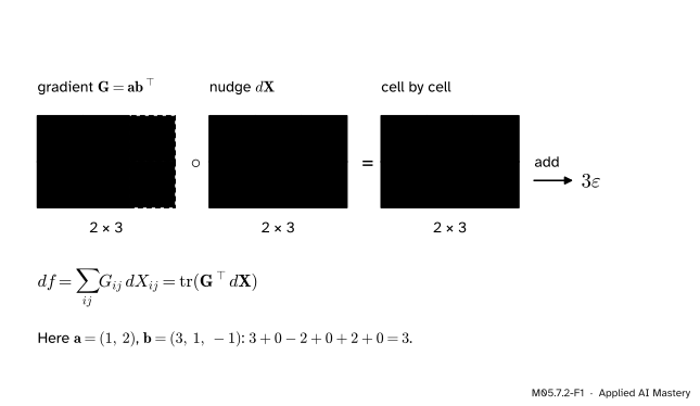
Nudge a matrix \(\mat{X}\) by a small matrix \(d\mat{X}\). A smooth function \(f\) changes by an amount \(df\) that, to first order, is a sum of one contribution from each entry: the size of the nudge there times how sensitive \(f\) is to that entry. The sensitivities form a matrix \(\mat{G}\) with the shape of \(\mat{X}\), and that matrix is the gradient.
M05.7.2-F1
The first-order change of \(f(\mat{X}) = \vect{a}\T\mat{X}\vect{b}\) for a 2 by 3 matrix \(\mat{X}\). Multiply the gradient and the nudge cell by cell and add: the total is \(df\).
“Multiply cell by cell and add” is the Frobenius inner product of two matrices of the same shape. It has a compact formula, \({\operatorname{tr}(\mat{G}\T d\mat{X})}\). So the method is: work out \(df\) with a few algebra rules, rearrange it into the form \({\operatorname{tr}(\mat{G}\T d\mat{X})}\), and read off \(\mat{G}\).
Build it up
Step 1. One variable. For \(f(x)\), the change is \(df = f'(x)\, dx\) to first order: the derivative is the number that multiplies \(dx\).
Step 2. A vector. For \(f(\vect{x})\), M05.2 showed that \(df = {\nabla f\T d\vect{x}}\): the gradient is the column whose dot product with \(d\vect{x}\) gives \(df\).
Step 3. A matrix. For \(f(\mat{X})\), the change is a sum over all entries,
\[
df = \sum_{i,j} G_{ij}\, dX_{ij} ,
\]
and \(\mat{G}\), the matrix of the \(G_{ij}\), is \(\nabla_{\mat{X}} f\).
Step 4. The sum is a trace. The diagonal entry \(j\) of \(\mat{G}\T d\mat{X}\) is \({(\mat{G}\T d\mat{X})_{jj}} = \sum_i G_{ij}\, dX_{ij}\), because row \(j\) of \(\mat{G}\T\) is column \(j\) of \(\mat{G}\). Adding the diagonal entries over \(j\) gives
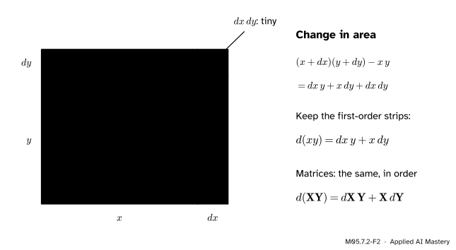
Step 5. Differentials of products. To find \(df\) we need the change of products of matrices. For numbers, the change in the area of an \(x\) by \(y\) rectangle is the picture.
M05.7.2-F2
The product rule. The two strips are first order in the nudge; the corner is a product of two small numbers, second order, and it is dropped.
For matrices the algebra is the same, except that the order of factors must be kept:
Dropping the second-order term leaves \({d(\mat{X}\mat{Y}) = d\mat{X}\,\mat{Y} + \mat{X}\,d\mat{Y}}\).
The formal statement
NoteThe differential method
If, for every small \(d\mat{X}\), \[
df = \operatorname{tr}(\mat{G}\T d\mat{X})
\] to first order, then \(\nabla_{\mat{X}} f = \mat{G}\). For a vector \(\vect{x}\) this reads \(df = \vect{g}\T d\vect{x}\) with \(\nabla f = \vect{g}\).
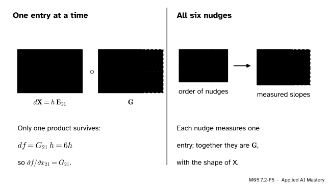
Why. Choose the nudge \(d\mat{X} = h\,\mat{E}_{ij}\), where \(\mat{E}_{ij}\) is the matrix with a 1 in row \(i\), column \(j\) and zeros elsewhere. Only one term of the sum in Step 4 survives, so \(df = G_{ij}\, h\), and the rate of change of \(f\) in entry \(x_{ij}\) is \(G_{ij}\). That is the definition of entry \((i, j)\) of the gradient.
M05.7.2-F5
Why the trace form gives the gradient, for \(f = \vect{a}\T\mat{X}\vect{b}\). A nudge of one entry picks out one entry of \(\mat{G}\); nudging every entry in turn measures all of it.
The rules. Each follows by writing out the change and keeping first-order terms. \(\mat{A}\) and \(\mat{B}\) are constant matrices.
Products: \(d(\mat{X}\mat{Y}) = d\mat{X}\,\mat{Y} + \mat{X}\,d\mat{Y}\), in this order (Step 5).
Transposes and traces: \(d(\mat{X}\T) = (d\mat{X})\T\) and \(d\operatorname{tr}(\mat{X}) = \operatorname{tr}(d\mat{X})\).
The trace tricks. A number is a \({1 \times 1}\) matrix, so it equals its own trace and its own transpose. A matrix and its transpose have the same diagonal, so \({\operatorname{tr}(\mat{M}\T)} = {\operatorname{tr}(\mat{M})}\). And the trace is cyclic: \({\operatorname{tr}(\mat{A}\mat{B}\mat{C})} = {\operatorname{tr}(\mat{C}\mat{A}\mat{B})}\), which is \({\operatorname{tr}(\mat{P}\mat{Q})} = {\operatorname{tr}(\mat{Q}\mat{P})}\) of M03.10.2 with \(\mat{P} = \mat{A}\mat{B}\) and \(\mat{Q} = \mat{C}\). Only cyclic moves are allowed: the order \(\mat{A}\mat{C}\mat{B}\) is a different product.
Gradient 1: \(f = \operatorname{tr}(\mat{A}\mat{X})\). By rules 1 and 4, \(df = \operatorname{tr}(\mat{A}\,d\mat{X})\). This is \({\operatorname{tr}(\mat{G}\T d\mat{X})}\) with \(\mat{G}\T = \mat{A}\), so \(\nabla_{\mat{X}} \operatorname{tr}(\mat{A}\mat{X}) = \mat{A}\T\).
Gradient 2: \(f = \vect{a}\T\mat{X}\vect{b}\). By rule 1, \(df = \vect{a}\T d\mat{X}\,\vect{b}\), a number. Take its trace and move \(\vect{b}\) to the front cyclically:
So \(\nabla_{\mat{X}}(\vect{a}\T\mat{X}\vect{b}) = \vect{a}\vect{b}\T\), which has the shape of \(\mat{X}\): \(\vect{a}\) has as many entries as \(\mat{X}\) has rows, and \(\vect{b}\) as many as it has columns. That answers the opening question.
Gradient 3: \(f = \norm{\mat{A}\mat{X} - \mat{B}}_F^2\). The squared Frobenius norm is the sum of the squares of all entries, \({\norm{\mat{R}}_F^2} = {\operatorname{tr}(\mat{R}\T\mat{R})}\). With \(\mat{R} = \mat{A}\mat{X} - \mat{B}\) we have \(d\mat{R} = \mat{A}\,d\mat{X}\), and
The first line is the product rule. The second uses \({\operatorname{tr}(d\mat{R}\T\mat{R})} = {\operatorname{tr}\big((\mat{R}\T d\mat{R})\T\big)} = {\operatorname{tr}(\mat{R}\T d\mat{R})}\). The third substitutes \(d\mat{R} = \mat{A}\,d\mat{X}\) and writes \({\mat{R}\T\mat{A}} = {(\mat{A}\T\mat{R})\T}\). So the gradient is \({2\mat{A}\T(\mat{A}\mat{X} - \mat{B})}\). With one column this is Identity 5 of M05.7.1.
Gradient 4: least squares. For the linear model with design matrix \(\mat{X}\) (one row per example, fixed) and weights \(\vect{w}\), the loss is \({L = \frac{1}{n}\vect{r}\T\vect{r}}\) with residual \(\vect{r} = \mat{X}\vect{w} - \vect{y}\). Now \(d\vect{r} = \mat{X}\,d\vect{w}\), and by the same two steps as Gradient 3,
So \(\nabla L = \tfrac{2}{n}\mat{X}\T(\mat{X}\vect{w} - \vect{y})\), the result M05.2.3 reached weight by weight. Setting it to zero gives the normal equations\({\mat{X}\T\mat{X}\,\vect{w}} = {\mat{X}\T\vect{y}}\) of M03.7.1.
Gradient 5: ridge. Ridge regression (ML01.9.1) adds the price \(\lambda\norm{\vect{w}}^2\). Its differential is \({2\lambda\,\vect{w}\T d\vect{w}}\), so the gradient gains the term \(2\lambda\vect{w}\):
Setting it to zero and multiplying by \(n/2\) gives \({(\mat{X}\T\mat{X} + n\lambda\mat{I})\,\vect{w}} = {\mat{X}\T\vect{y}}\). As in ML01.9.1, the penalty is applied to centred data without a bias, because the bias is not penalised.
Worked example
Use the running loss. The design matrix has the column \(\vect{x} = (1, 2, 3, 4)\) and a column of ones, the targets are \(\vect{y} = (2, 3, 5, 6)\), \(n = 4\), and the parameters are \((w, b)\). First the two products that appear everywhere:
For example \(30 = 1 + 4 + 9 + 16\) and \(47 = 2 + 6 + 15 + 24\).
M05.7.2-F3
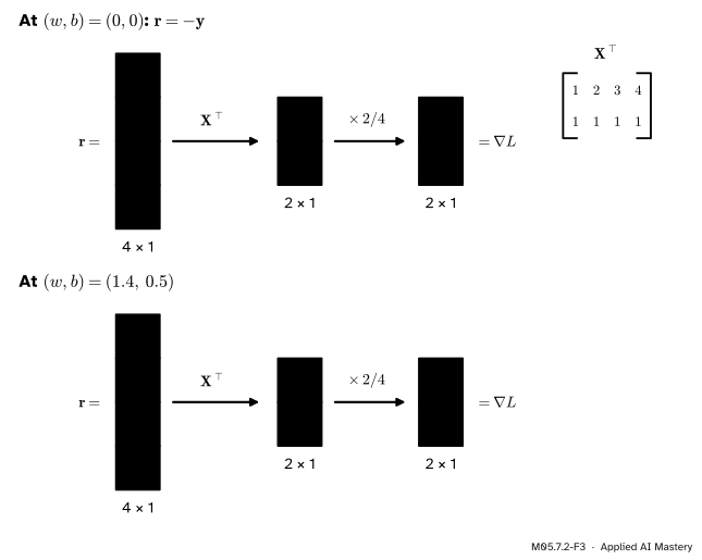
The gradient \({\tfrac{2}{n}\mat{X}\T\vect{r}}\) of the running loss at two points. The residual has one entry per example; \(\mat{X}\T\) turns it into one entry per parameter.
At the origin.\(\mat{X}\vect{w} = \vect{0}\), so \(\vect{r} = -\vect{y} = (-2, -3, -5, -6)\), and
so \(\nabla L = \tfrac{2}{4}(-47, -16) = (-23.5, -8)\), as M04.10 found.
At \((1.4, 0.5)\). The predictions are \((1.9, 3.3, 4.7, 6.1)\), so \(\vect{r} = (-0.1, 0.3, -0.3, 0.1)\). Then the first entry of \(\mat{X}\T\vect{r}\) is \({-0.1 + 0.6 - 0.9 + 0.4} = 0\) and the second is \({-0.1 + 0.3 - 0.3 + 0.1} = 0\). The gradient is zero: this is the lowest point.
The normal equations by hand.\(30w + 10b = 47\) and \(10w + 4b = 16\). The determinant is \({30 \cdot 4 - 10 \cdot 10} = 20\), so
Ridge. Centre the data as ML01.9.1 does: \(\vect{z} = \vect{x} - 2.5 = (-1.5, -0.5, 0.5, 1.5)\) and \(\vect{y} - 4 = (-2, -1, 1, 2)\). Then \({\vect{z}\T\vect{z}} = 5\) and the product with the centred targets is \(3 + 0.5 + 0.5 + 3 = 7\). With \(\lambda = 0.5\) the ridge equation is \({(5 + 4 \cdot 0.5)\,w} = 7\), so \(w = 1\): the slope ML01.9.1 found for that price, down from 1.4.
Code
From scratch: a gradient with respect to a matrix by central differences, one entry at a time, checked against Gradients 1 to 3 on random matrices.
import numpy as npdef num_grad(f, X, h=1e-6):"""Central differences, one entry of X at a time: a matrix with the shape of X.""" G = np.zeros_like(X, dtype=float)for index in np.ndindex(X.shape): E = np.zeros_like(X, dtype=float) E[index] = h G[index] = (f(X + E) - f(X - E)) / (2* h)return Grng = np.random.default_rng(3)X = rng.normal(size=(2, 3))A3, A2 = rng.normal(size=(3, 2)), rng.normal(size=(4, 2))a, b, B = rng.normal(size=2), rng.normal(size=3), rng.normal(size=(4, 3))cases = {"tr(AX)": (lambda M: np.trace(A3 @ M), A3.T),"a^T X b": (lambda M: a @ M @ b, np.outer(a, b)),"||AX - B||_F^2": (lambda M: np.sum((A2 @ M - B) **2), 2* A2.T @ (A2 @ X - B)),}gaps = {}for name, (f, G) in cases.items(): numeric = num_grad(f, X)assert numeric.shape == G.shape == X.shape gaps[name] = np.abs(numeric - G).max()print(f"{name:15s} shape {G.shape} largest gap {gaps[name]:.1e}")
tr(AX)          shape (2, 3)   largest gap 2.0e-10
a^T X b         shape (2, 3)   largest gap 3.0e-11
||AX - B||_F^2  shape (2, 3)   largest gap 2.1e-09
Now the running loss: the gradient formula, the normal equations, and ridge, first from the formula and then with scikit-learn. Its Ridge minimises \({\norm{\vect{y} - \mat{X}\vect{w}}^2 + \alpha\norm{\vect{w}}^2}\) without the factor \(1/n\), so our price \(\lambda\) corresponds to \(\alpha = n\lambda\), and it fits an unpenalised intercept.
from sklearn.linear_model import Ridgex = np.array([1.0, 2.0, 3.0, 4.0])y = np.array([2.0, 3.0, 5.0, 6.0])D = np.column_stack([x, np.ones(4)]) # the design matrix of the running lossn =len(y)grad =lambda w: 2/ n * D.T @ (D @ w - y)print("X^T X =", (D.T @ D).tolist(), " X^T y =", (D.T @ y).tolist())print("gradient at the origin:", grad(np.zeros(2)), " at (1.4, 0.5):", grad(np.array([1.4, 0.5])).round(12))w_star = np.linalg.solve(D.T @ D, D.T @ y)print("normal equations:", w_star)lam =0.5z, yc = x - x.mean(), y - y.mean()w_ridge = (z @ yc) / (z @ z + n * lam)model = Ridge(alpha=n * lam).fit(x.reshape(-1, 1), y)print("ridge slope from the formula:", w_ridge, " scikit-learn:", model.coef_, model.intercept_)
X^T X = [[30.0, 10.0], [10.0, 4.0]]   X^T y = [47.0, 16.0]
gradient at the origin: [-23.5  -8. ]   at (1.4, 0.5): [-0. -0.]
normal equations: [1.4 0.5]
ridge slope from the formula: 1.0   scikit-learn: [1.] 1.5
The intercept is \({4 - 1 \cdot 2.5} = 1.5\): the centred fit moved back to the original units.
Explore
M05.7-X1
Gradient heatmap
Pick a function of a small matrix \(\mat{X}\) and move its entries with the sliders. Each cell on the left is the slope measured by nudging that entry; each cell on the right is the formula. Switch to the common mistake and watch the shapes or the values stop matching.
Pitfalls
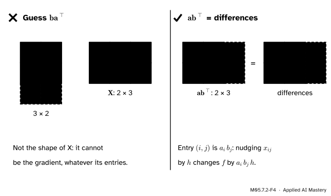
M05.7.2-F4
Wrong beside right for the gradient of \(\vect{a}\T\mat{X}\vect{b}\) with \(\vect{a} = (1, 2)\), \(\vect{b} = (3, 1, -1)\) and \(\mat{X}\) of shape 2 by 3. The shape alone rules out the guess.
“The gradient of \(\vect{a}\T\mat{X}\vect{b}\) is \(\vect{b}\vect{a}\T\).”
That is its transpose. The quickest check is the shape: the gradient must have the shape of \(\mat{X}\). For a square \(\mat{X}\) the shapes agree and only the numbers can tell, so check one entry: nudging \(x_{ij}\) changes \(f\) by \(a_i b_j\) times the nudge.
“\(d(\mat{X}\T\mat{X}) = 2\mat{X}\T d\mat{X}\).”
The product rule keeps the order: \({d(\mat{X}\T\mat{X})} = {d\mat{X}\T\,\mat{X} + \mat{X}\T d\mat{X}}\). The two terms are transposes of each other, not equal. Only after taking a trace, as in Gradient 3, do they contribute the same amount.
“Inside a trace I can reorder freely.”
Only cyclically. \({\operatorname{tr}(\mat{A}\mat{B}\mat{C})} = {\operatorname{tr}(\mat{B}\mat{C}\mat{A})}\), but \({\operatorname{tr}(\mat{A}\mat{C}\mat{B})}\) is in general a different number, and for rectangular matrices it may not even be defined.
Check yourself
Recall
1. If \(df = \operatorname{tr}(\mat{G}\T d\mat{X})\) for every \(d\mat{X}\), what is \(\nabla_{\mat{X}} f\)?
Show answer
\(\mat{G}\).
2. State the product rule for differentials of matrices.
Show answer
\(d(\mat{X}\mat{Y}) = d\mat{X}\,\mat{Y} + \mat{X}\,d\mat{Y}\), keeping the order of the factors.
3. What is the gradient of \(\operatorname{tr}(\mat{A}\mat{X})\)?
Show answer
\(\mat{A}\T\).
4. What is the gradient of \(\vect{a}\T\mat{X}\vect{b}\)?
Show answer
\(\vect{a}\vect{b}\T\), which has the shape of \(\mat{X}\).
5. What are the normal equations, and where do they come from?
Show answer
\({\mat{X}\T\mat{X}\,\vect{w}} = {\mat{X}\T\vect{y}}\): the gradient \({\tfrac{2}{n}\mat{X}\T(\mat{X}\vect{w} - \vect{y})}\) of the mean squared error set to zero.
Exercises
1.★ Use differentials to find the gradient of \(f(\mat{X}) = \operatorname{tr}(\mat{X}\T\mat{A})\).
Show solution
\(df = \operatorname{tr}(d\mat{X}\T\mat{A})\). A matrix and its transpose have the same trace, so \(df = {\operatorname{tr}(\mat{A}\T d\mat{X})}\), which is \({\operatorname{tr}(\mat{G}\T d\mat{X})}\) with \(\mat{G} = \mat{A}\). So \(\nabla_{\mat{X}} f = \mat{A}\).
2.★★ Find the gradient of \(f(\mat{X}) = \norm{\mat{X}}_F^2\) and of \(g(\mat{X}) = \vect{a}\T\mat{X}\T\vect{b}\).
Show solution
\(f = \operatorname{tr}(\mat{X}\T\mat{X})\), so \(df = {\operatorname{tr}(d\mat{X}\T\mat{X})} + {\operatorname{tr}(\mat{X}\T d\mat{X})} = {2\operatorname{tr}(\mat{X}\T d\mat{X})}\), and \(\nabla f = 2\mat{X}\). For \(g\), \(dg = \vect{a}\T d\mat{X}\T\vect{b}\), a number, equal to its own transpose \(\vect{b}\T d\mat{X}\,\vect{a}\). By Gradient 2 with the roles of \(\vect{a}\) and \(\vect{b}\) swapped, \(\nabla g = \vect{b}\vect{a}\T\).
3.★★★ Weighted least squares gives example \(i\) a weight \(c_i > 0\): \(L(\vect{w}) = (\mat{X}\vect{w} - \vect{y})\T\mat{C}(\mat{X}\vect{w} - \vect{y})\) with \(\mat{C} = \operatorname{diag}(c_1, \dots, c_n)\). Derive the gradient and the equations for the minimum.
Show solution
With \(\vect{r} = \mat{X}\vect{w} - \vect{y}\), \(L = \vect{r}\T\mat{C}\vect{r}\) and \(d\vect{r} = \mat{X}\,d\vect{w}\). The product rule gives
where the two terms are equal because the first is a number, equal to its transpose \(\vect{r}\T\mat{C}\T d\vect{r}\), and \(\mat{C}\) is symmetric. So \(\nabla L = 2\mat{X}\T\mat{C}(\mat{X}\vect{w} - \vect{y})\), and the minimum solves \({\mat{X}\T\mat{C}\mat{X}\,\vect{w}} = {\mat{X}\T\mat{C}\vect{y}}\).
Summary card
Write \(df\), make it \(\operatorname{tr}(\mat{G}\T d\mat{X})\), read off \(\mat{G}\).
Least squares:\(\nabla L = \tfrac{2}{n}\mat{X}\T(\mat{X}\vect{w} - \vect{y})\), plus \(2\lambda\vect{w}\) for ridge.
Sources and next steps
Sources. Each was opened and checked against this lesson on 15 November 2026.
Paige Bright, Alan Edelman and Steven G. Johnson, Matrix Calculus (for Machine Learning and Beyond), course notes of MIT 18.S096: Theorem 2 in Section 1.3, the product rule \(d(\mat{A}\mat{B}) = d\mat{A}\,\mat{B} + \mat{A}\,d\mat{B}\); Section 5.1, Definition 34 (the Frobenius inner product \(\operatorname{tr}(\mat{A}\T\mat{B})\), so that the gradient is defined by \(df = \operatorname{tr}((\nabla f)\T d\mat{A})\)) and Example 36 (\(\nabla(\vect{x}\T\mat{A}\vect{y}) = \vect{x}\vect{y}\T\)).
Kaare Brandt Petersen and Michael Syskind Pedersen, The Matrix Cookbook, version of 15 November 2012: the rules (33) to (37) and (44) at the start of Section 2; (70) for \(\vect{a}\T\mat{X}\vect{b}\); (100) for \(\operatorname{tr}(\mat{X}\mat{A})\); and (132) for the Frobenius norm.
Marc Peter Deisenroth, A. Aldo Faisal and Cheng Soon Ong, Mathematics for Machine Learning, Section 5.5, (5.106): \(\partial(\vect{a}\T\mat{X}\vect{b})/\partial\mat{X} = \vect{a}\vect{b}\T\).
scikit-learn, sklearn.linear_model.Ridge: the objective \({\norm{\vect{y} - \mat{X}\vect{w}}^2 + \alpha\norm{\vect{w}}^2}\) and fit_intercept.