A hand-derived gradient can be wrong and still look plausible. Probe the function twice along every axis, compare the two gradients by their relative error, choose the step that balances truncation against rounding, and catch the bugs, at a cost of 2n evaluations.
M05.2.4L2 Intermediate25 minIn review (what this means)
The maths and code on this page are checked by automated tests on every change, but an independent reader has not signed it off yet. Spot a mistake or a confusing step? Tell us.
Compute a numerical gradient by central differences in each coordinate, 2n evaluations of f, and derive its error of order h².
Compare two gradients by the relative error ‖g₁ − g₂‖ / (‖g₁‖ + ‖g₂‖) and read it against the thresholds used in practice.
Explain why a step near 10⁻⁵ works best in double precision, from the balance of truncation and rounding.
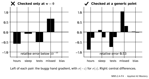
Catch a deliberately wrong hand gradient, find the weight it gets wrong, and explain why a check at w = 0 can miss a bug.
Use scipy.optimize.approx_fprime and scipy.optimize.check_grad, knowing that both use forward differences and that check_grad returns an absolute error.
The question
The last lesson derived \({\tfrac1n\mat{X}\T(\vect{p} - \vect{y})}\) by hand. Suppose your code for it has a slip: a missing \({\tfrac1n}\), a wrong sign. Training still runs, the loss may even fall a little, and nothing crashes. How can you test a gradient formula against the function itself, and how small must the disagreement be before you trust it?
From the last lesson
1. What is the gradient of the mean squared error \({\tfrac1n\norm{\mat{X}\vect{w} - \vect{y}}^2}\)?
Show answer
\({\tfrac2n\mat{X}\T(\mat{X}\vect{w} - \vect{y})}\), one entry per weight.
2. What is the derivative of one example’s log loss with respect to its score?
Show answer
\({p - y}\): the predicted probability minus the label.
Intuition
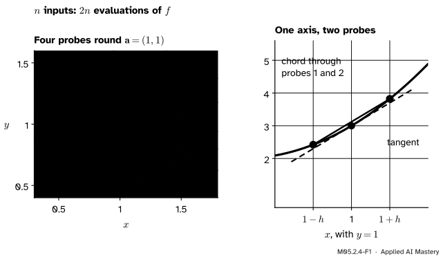
The definition of a partial derivative is a recipe a computer can follow: move one input a tiny amount, see how much \(f\) changes, divide. Do it forwards and backwards along each axis, and the chord through the two probes has nearly the slope of the tangent. With \(n\) inputs that is \({2n}\) evaluations of \(f\) and no calculus at all.
M05.2.4-F1
A numerical gradient. Two probes per axis, four for two inputs. The chord through the probes on each axis estimates that partial derivative; for this quadratic slice it is exactly parallel to the tangent.
That number is a second opinion that knows nothing about your derivation. If the formula and the probes agree to many digits, the formula is almost certainly right. If they disagree, the probes also tell you which weight is wrong.
Build it up
Step 1. The estimate and its error. Along axis \(i\) the central difference is
Since \({s'(0) = \pd{f}{x_i}(\vect{a})}\), the error is of order \({h^2}\), as M04.2.4 found in one variable. For a quadratic, \({s''' = 0}\) and the central difference is exact, which is why the chord in the figure is parallel to the tangent.
Step 2. One number for the disagreement. The two gradients are vectors. Their difference \({\norm{\vect{g}_1 - \vect{g}_2}}\) alone is no use: \({10^{-3}}\) is tiny next to a gradient of length 1000 and huge next to one of length \({10^{-4}}\). Divide by the sizes instead. The relative error is
\[
e = \frac{\norm{\vect{g}_1 - \vect{g}_2}}{\norm{\vect{g}_1} + \norm{\vect{g}_2}} .
\]
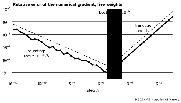
Step 3. Choose the step. A smaller \(h\) shrinks the \({h^2}\) error, but every value of \(f\) carries a rounding error of about \({10^{-16}}\) times its size, and dividing a difference by \({2h}\) magnifies it to about \({10^{-16}/h}\). One error falls as \(h\) shrinks and the other grows.
M05.2.4-F2
The relative error of a central-difference gradient against the exact one, for the five-weight log loss of the worked example. Right of the minimum the \({h^2}\) truncation error rules; left of it, rounding.
The best step makes the two about equal. Setting \({h^2 \approx 10^{-16}/h}\) gives \({h^3 \approx 10^{-16}}\), so \({h}\) near \({10^{-5}}\) in double precision: the value CS231n recommends. The exact best step depends on the function and the platform; the lesson’s figure is one machine’s run.
The formal statement
NoteDefinitions: numerical gradient and relative error
For \({f : \R^n \to \R}\) and a step \({h > 0}\), the central-difference gradient at \(\vect{a}\) has entries
for \({i = 1, \dots, n}\), which costs \({2n}\) evaluations of \(f\). The relative error between two gradients \(\vect{g}_1\) and \(\vect{g}_2\), not both zero, is
\[
e = \frac{\norm{\vect{g}_1 - \vect{g}_2}}{\norm{\vect{g}_1} + \norm{\vect{g}_2}} .
\]
Three properties make \(e\) easy to read.
It lies between 0 and 1. By the triangle inequality, \({\norm{\vect{g}_1 - \vect{g}_2} \le \norm{\vect{g}_1} + \norm{\vect{g}_2}}\). It is 0 only when the gradients are equal.
It reaches 1 for opposite gradients. If \({\vect{g}_2 = -\vect{g}_1}\), the top is \({2\norm{\vect{g}_1}}\) and so is the bottom: a sign error gives \({e = 1}\).
It ignores scale. Multiplying both gradients by the same \({c > 0}\) multiplies top and bottom by \(c\). A factor \(k\) in one of them gives \({\abs{k - 1}/(\abs{k} + 1)}\), so a missing \({\tfrac1n}\) with \({n = 6}\), which multiplies the whole gradient by 6, gives \({5/7 \approx 0.71}\).
In practice, with \({h \approx 10^{-5}}\) in double precision, CS231n reads a relative error like this: above \({10^{-2}}\) the gradient is probably wrong; between \({10^{-4}}\) and \({10^{-2}}\) is suspicious; below \({10^{-4}}\) is usually fine for a function with kinks, such as ReLU; and \({10^{-7}}\) or less is good. (CS231n divides by the larger of the two sizes rather than their sum, which changes the value by at most a factor of 2, and applies the measure entry by entry, so its lines are rough guides for the single number used here.)
M05.2.4-F5
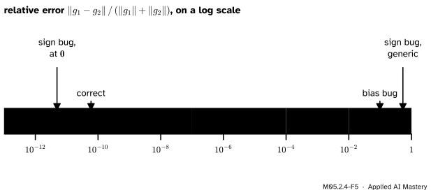
The four checks of this lesson on the scale of relative error. Notice the second arrow: a buggy gradient that scores as well as a correct one, because it was checked at \({\vect{w} = \vect{0}}\).
The cost. Each of the \({2n}\) evaluations runs the whole model on the data. For a network with \({10^6}\) weights a single numerical gradient takes \({2 \times 10^6}\) forward passes. That is why numerical gradients are a test, run on a small model or a few weights, and never the way a network is trained. Reverse-mode differentiation (M05.8) delivers the whole gradient for a small constant multiple of one evaluation.
Worked example
A check with five weights. Give each of the six students of M05.2.3 four features (hours studied, hours slept, practice tests taken and lectures missed) and a bias, so \({n = 6}\) examples and five weights. The hand gradient of the mean log loss is \({\tfrac16\mat{X}\T(\vect{p} - \vect{y})}\). Check it at \({\vect{w} = (0.3, -0.2, 0.4, -0.3, 0.1)}\) with \({h = 10^{-5}}\).
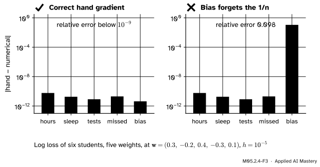
and their relative error is below \({10^{-9}}\): good.
Now plant a bug: the bias entry forgets the \({\tfrac1n}\), so it is multiplied by 6, from \(-0.0222\) to \(-0.1333\). The other four entries are untouched. The difference vector is \({(0, 0, 0, 0, -0.1111)}\) to ten digits, so the top of the relative error is 0.111, and the bottom is about \({0.557 + 0.572}\). The relative error is about 0.098: probably wrong.
M05.2.4-F3
The check weight by weight. With the correct formula every gap is at rounding level. With the bug, four gaps stay there and one leaps to about 0.1: the check names the faulty entry.
The single number says that something is wrong; the entries say where. A tall bar on the bias alone points straight at the bias line of the code.
Code
From scratch first: the numerical gradient, the relative error, and a check that reports the worst weight.
The correct gradient passes with a relative error below \({10^{-9}}\), the bias bug fails at about 0.098 and points at weight 4 (the bias, counting from 0), and the sign bug fails at about 0.5. Yet at \({\vect{w} = \vect{0}}\) the sign bug passes. Next, the step size: the sweep below shows the \({h^2}\) regime and the rounding regime.
for h in (1e-1, 1e-2, 1e-3, 1e-5, 1e-8, 1e-11):print(f"h = {h:.0e}: relative error {relative_error(grad(w), numerical_gradient(loss, w, h)):.1e}")
h = 1e-01: relative error 6.2e-03
h = 1e-02: relative error 6.2e-05
h = 1e-03: relative error 6.2e-07
h = 1e-05: relative error 5.9e-11
h = 1e-08: relative error 7.3e-09
h = 1e-11: relative error 6.1e-06
From \({h = 10^{-2}}\) to \({10^{-3}}\) the error falls about a hundredfold, the \({h^2}\) law; at \({10^{-11}}\) it is far worse than at \({10^{-5}}\). SciPy has both halves of the check ready-made. scipy.optimize.approx_fprime returns a numerical gradient and scipy.optimize.check_grad compares it with your function. Both use forward differences with a step of about \({1.49 \times 10^{-8}}\), and check_grad returns the absolute norm of the difference, not a relative error.
from scipy.optimize import approx_fprime, check_gradapprox = approx_fprime(w, loss)print("approx_fprime vs hand, relative error: %.1e"% relative_error(grad(w), approx))print("check_grad, correct: %.1e bias bug: %.4f"% (check_grad(loss, grad, w), check_grad(loss, grad_bias_bug, w)))
The forward differences are less accurate than ours, about \({10^{-8}}\) instead of \({10^{-10}}\), but still far below the warning lines. To read check_grad on the relative scale, divide its result by \({\norm{\vect{g}_1} + \norm{\vect{g}_2}}\) yourself.
Explore
This module’s interactive lives in lesson M05.2.2. A numerical gradient is a linear model fitted from probes, so shrink the step there and watch the remainder vanish: that vanishing is what makes small probes trustworthy.
Pitfalls
M05.2.4-F4
Wrong beside right. At \({\vect{w} = \vect{0}}\) every score is 0, where \({\sigma(-z) = \sigma(z) = \tfrac12}\), so the buggy gradient is exactly the true one there. At a generic point the bug shows at once.
“The check passed at the starting point, so the gradient is right.”
Starting points are special. At \({\vect{w} = \vect{0}}\) every probability is \({\tfrac12}\), and any bug that only changes how \(\vect{p}\) depends on \(\vect{z}\) is invisible. Check at a random point, or at one reached after a few training steps; CS231n recommends checking during a “characteristic mode of operation” for the same reason.
“A smaller step always gives a better numerical gradient.”
Below about \({10^{-5}}\) rounding error grows like \({10^{-16}/h}\). With \({h = 10^{-11}}\) the five-weight check is worse than at \({10^{-5}}\) by a factor of more than a hundred. In single precision, where rounding is about \({10^{-7}}\), the trouble starts much sooner: check in double precision.
“check_grad returned 0.11, so the gradient is 11% off.”
check_grad returns \({\norm{\vect{g}_1 - \vect{g}_2}}\), an absolute size. A value of 0.11 is a disaster for a gradient of length 0.5 and harmless for one of length \({10^4}\). Divide by the sizes, or compute the relative error yourself.
Check yourself
Recall
1. How many evaluations of \(f\) does a central-difference gradient of \({f : \R^n \to \R}\) take?
Show answer
\({2n}\): two for each input.
2. What is the order of the central difference’s truncation error, and when is it exact?
Show answer
Order \({h^2}\), with leading term \({\tfrac{h^2}{6}s'''(0)}\); it is exact when the third derivative of the slice is 0, for example for any quadratic.
3. Write the relative error between \(\vect{g}_1\) and \(\vect{g}_2\), and say what value a sign error gives.
Show answer
\({\norm{\vect{g}_1 - \vect{g}_2}/(\norm{\vect{g}_1} + \norm{\vect{g}_2})}\); for \({\vect{g}_2 = -\vect{g}_1}\) it is 1.
4. Why does a step near \({10^{-5}}\) work best in double precision?
Show answer
Truncation error falls like \({h^2}\) and rounding error grows like \({10^{-16}/h}\); they balance where \({h^3 \approx 10^{-16}}\), near \({h = 10^{-5}}\).
5. Why are numerical gradients not used to train large networks?
Show answer
They need \({2n}\) evaluations of the loss, two million for a million weights, while reverse-mode differentiation gives the whole gradient for a small multiple of one evaluation.
Exercises
1.★ A hand gradient is \({(3, 4)}\) and a numerical one is \({(3, 4.1)}\). Compute the relative error and say how to read it.
Show solution
The difference is \({(0, -0.1)}\), of norm 0.1. The norms are 5 and \({\sqrt{9 + 16.81} = \sqrt{25.81} \approx 5.080}\). So \({e \approx 0.1/10.080 \approx 0.0099}\): just under \({10^{-2}}\), in the suspicious band and close to probably wrong. With \({h = 10^{-5}}\) a correct formula should do far better, so look for a bug in the second entry.
2.★★ Find the error of the forward difference \({(f(\vect{a} + h\vect{e}_i) - f(\vect{a}))/h}\) to leading order, and explain why approx_fprime uses a step near \({10^{-8}}\) rather than \({10^{-5}}\).
Show solution
With the slice \(s\) as in Step 1, \({s(h) \approx s(0) + hs'(0) + \tfrac{h^2}{2}s''(0)}\), so the forward difference is \({s'(0) + \tfrac{h}{2}s''(0)}\): an error of order \(h\), not \({h^2}\). Rounding still contributes about \({10^{-16}/h}\). The two balance where \({h \approx 10^{-16}/h}\), that is \({h^2 \approx 10^{-16}}\) and \({h \approx 10^{-8}}\), which is the square root of the machine epsilon, the default of approx_fprime. The best accuracy is then about \({10^{-8}}\), against \({10^{-10}}\) or better for central differences.
3.★★★ A hand gradient \(\vect{g}_2\) equals the true gradient \(\vect{g}_1\) in every entry but one, where it is off by \(\delta\). Show that the relative error is at least \({\abs{\delta}/(2\norm{\vect{g}_1} + \abs{\delta})}\), and use it to explain why a single wrong entry in a gradient with a million entries can still be caught.
Show solution
The top is exactly \({\norm{\vect{g}_1 - \vect{g}_2} = \abs{\delta}}\). By the triangle inequality \({\norm{\vect{g}_2} \le \norm{\vect{g}_1} + \abs{\delta}}\), so the bottom is at most \({2\norm{\vect{g}_1} + \abs{\delta}}\), and \({e \ge \abs{\delta}/(2\norm{\vect{g}_1} + \abs{\delta})}\). The bound depends on the size of the gradient, not on the number of entries. If one entry of a gradient of length 1 is off by 0.01, then \({e \ge 0.01/2.01 \approx 0.005}\), far above the \({10^{-7}}\) of a correct formula, however many entries there are. Rounding noise grows with \(n\) only slowly, so the bug still stands out; the per-entry gaps then point at it, as in the worked example.
Summary card
Probe twice per axis; trust a gradient only when the relative error is tiny at a generic point.
M05.2.4-F1
Two probes per axis, 2n in all.
Central difference. Two probes per axis, \({2n}\) evaluations, error about \({\tfrac{h^2}{6}s'''}\).
Relative error.\({\norm{\vect{g}_1 - \vect{g}_2}/(\norm{\vect{g}_1} + \norm{\vect{g}_2})}\), between 0 and 1.
Read it. Below \({10^{-7}}\) good; above \({10^{-2}}\) probably wrong.
Step.\({h \approx 10^{-5}}\) in double precision.
Where. A generic point, not \({\vect{w} = \vect{0}}\).
Sources and next steps
Sources. Each was opened and checked against this lesson on 15 November 2026.
CS231n, Neural Networks Part 3: Learning and Evaluation, section Gradient Checks: use the centred formula with \(h\) about \({10^{-5}}\); compare by a relative error that divides by the larger of the two sizes; relative error above \({10^{-2}}\) “usually means the gradient is probably wrong”, between \({10^{-2}}\) and \({10^{-4}}\) “should make you feel uncomfortable”, below \({10^{-4}}\) “is usually okay for objectives with kinks”, and \({10^{-7}}\) or less “you should be happy”; use double precision; beware kinks; check during a “characteristic mode of operation”.
Marc Peter Deisenroth, A. Aldo Faisal and Cheng Soon Ong, Mathematics for Machine Learning, the remark “Verifying the Correctness of a Gradient Implementation” at the end of Section 5.2.2: compare a finite-difference approximation with a step such as \({10^{-4}}\) against the analytic gradient, with a measure built from the entrywise differences and sums of the two gradients below \({10^{-6}}\).
SciPy 1.18 reference, scipy.optimize.approx_fprime (the forward finite difference formula, default step the square root of the machine epsilon, about \({1.49 \times 10^{-8}}\)) and scipy.optimize.check_grad (returns the 2-norm of the difference between the given gradient and the finite-difference approximation; direction="all" by default).
Next. Module M05.3, Directional derivatives and steepest ascent, uses the linear model to find the slope in any direction. M05.8 replaces the \({2n}\) probes with automatic differentiation, and M05.9.3 runs this check on a whole network.