Differentiate every partial derivative again and you get n squared second partial derivatives. Stack them into the Hessian, the Jacobian of the gradient, see why it is symmetric, meet the function where it is not, and compute it by hand, by finite differences and with SciPy.
M05.5.1L2 Intermediate25 minIn review (what this means)
The maths and code on this page are checked by automated tests on every change, but an independent reader has not signed it off yet. Spot a mistake or a confusing step? Tell us.
Compute every second partial derivative of a function of several inputs and arrange them in the Hessian matrix.
Explain the Hessian as the Jacobian of the gradient: column j says how the gradient changes per unit step along input j.
State Schwarz’s theorem on mixed partial derivatives, follow its proof, and use Peano’s function to show why its hypothesis matters.
Compute a Hessian by central differences of the gradient and check it with scipy.differentiate.hessian.
The question
At the origin the gradient of the running loss is \({(-23.5, -8)}\): it says which way is uphill and how steep the climb is. Take one step and the gradient is different. How fast does the gradient itself change, and does it change at the same rate in every direction? The answer is a matrix of second derivatives, and every method that is smarter than plain gradient descent, from Newton’s method to the rule that caps the learning rate, is built on it.
Intuition
The gradient is an arrow attached to every point. Move the point and the arrow turns and stretches. The quickest way to see how is to take one small step along each input and compare the arrows.
M05.5.1-F1
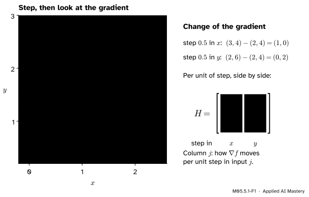
Step from \({(1, 1)}\) along \(x\) and the gradient of the running bowl changes only in its first entry; step along \(y\) and only the second changes, twice as fast. Those two changes per unit of step, side by side, are the Hessian.
For the running bowl \({f(x, y) = x^2 + 2y^2}\) the gradient is \({(2x, 4y)}\). A step of 0.5 along \(x\) moves it from \({(2, 4)}\) to \({(3, 4)}\), a change of \({(1, 0)}\), or \({(2, 0)}\) per unit of step. A step of 0.5 along \(y\) moves it to \({(2, 6)}\), a change of \({(0, 4)}\) per unit. Stand the two changes up as columns and you have a \({2 \times 2}\) matrix, the Hessian. It is to the gradient what the derivative is to a function: its rate of change.
The two columns are not equal. Along \(y\) the gradient grows twice as fast, because the bowl curves up twice as sharply in that direction. That is the first hint of what the Hessian measures: curvature, and how it differs from one direction to another.
Build it up
Step 1. A partial derivative is a function too. For the running loss
the two partial derivatives are \({\pd{L}{w} = 15w + 5b - 23.5}\) and \({\pd{L}{b} = 5w + 2b - 8}\). Each is a new function of \(w\) and \(b\), with slopes of its own.
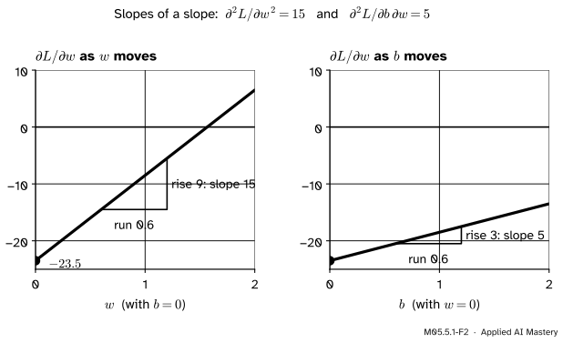
Step 2. Differentiate each one again, along each input. The slope of \({\pd{L}{w}}\) as \(w\) moves is 15. Its slope as \(b\) moves is 5. A second partial derivative is the slope of a slope.
M05.5.1-F2
The partial derivative \({\pd{L}{w}}\) is a straight line in each input. Its slope along \(w\) is 15 and its slope along \(b\) is 5: two second partial derivatives of the running loss.
Step 3. Name the four results. Differentiating \({\pd{L}{b}}\) the same way gives 5 along \(w\) and 2 along \(b\). Write \({L_{ww} = 15}\), \({L_{wb} = 5}\), \({L_{bw} = 5}\) and \({L_{bb} = 2}\), where the subscripts list the inputs in the order you differentiate: \(L_{wb}\) means “first along \(w\), then along \(b\)”.
Step 4. Stack them. Put the slopes of \({\pd{L}{w}}\) in row 1 and the slopes of \({\pd{L}{b}}\) in row 2:
The diagonal entries say how sharply the loss curves along each input on its own. The off-diagonal 5 comes from the term \({5wb}\): it says how the slope in \(w\) changes when \(b\) moves. The running bowl has no \({xy}\) term, so its Hessian \({\begin{bmatrix} 2 & 0 \\ 0 & 4 \end{bmatrix}}\) has zeros off the diagonal.
The formal statement
NoteDefinition: second partial derivatives and the Hessian
Let \({f : \R^n \to \R}\) have partial derivatives that themselves have partial derivatives at \(\vect{a}\). The second partial derivative along \(x_i\) and then \(x_j\) is
The Hessian\(\mat{H}_f(\vect{a})\), also written \({\nabla^2 f(\vect{a})}\), is the \({n \times n}\) matrix whose entry in row \(i\) and column \(j\) is that number.
Row \(i\) of the Hessian holds the partial derivatives of the single function \({\pd{f}{x_i}}\), which is output \(i\) of the gradient map \({\vect{x} \mapsto \nabla f(\vect{x})}\). In the numerator layout of M05.4, row \(i\) of a Jacobian is the transposed gradient of output \(i\). So
Column \(j\) is \({\mat{H}\vect{e}_j}\), the change of the gradient per unit step along input \(j\): exactly the picture of the anchor figure. For the bowl the gradient is linear, so the approximation is exact: \({(2, 4) + \mat{H}\,(0.5, 0) = (3, 4)}\).
Are the two mixed entries always equal? In every example so far, yes. The theorem below says when that is guaranteed.
NoteTheorem: symmetry of second derivatives (Schwarz, also called Clairaut)
If all the second partial derivatives of \(f\) exist and are continuous on an open ball around \(\vect{a}\), then for every \(i\) and \(j\)
Symmetry is what makes the Hessian so useful. By the spectral theorem (M03.3) a symmetric matrix has real eigenvalues and perpendicular eigenvectors, and the next two lessons read curvature off exactly those.
Go deeper: the proof, by a double difference quotient
Take two inputs, a point \({(a, b)}\), and small steps \({h, k \neq 0}\). Form the double difference
\[
\begin{aligned}
\Delta &= f(a + h, b + k) - f(a + h, b) \\
&\quad - f(a, b + k) + f(a, b) .
\end{aligned}
\]
First grouping. Let \({g(x) = f(x, b + k) - f(x, b)}\), so that \({\Delta = g(a + h) - g(a)}\). By the mean value theorem there is a \(\xi\) between \(a\) and \({a + h}\) with
\[
\begin{aligned}
\Delta &= h\, g'(\xi) \\
&= h \big( f_x(\xi, b + k) - f_x(\xi, b) \big) .
\end{aligned}
\]
The bracket is a change of the function \({y \mapsto f_x(\xi, y)}\), so the mean value theorem again gives an \(\eta\) between \(b\) and \({b + k}\) with \({\Delta = hk\, f_{xy}(\xi, \eta)}\).
Second grouping. Let \({p(y) = f(a + h, y) - f(a, y)}\), so that \({\Delta = p(b + k) - p(b)}\). The same two steps, in the other order, give points \(\xi'\) and \(\eta'\) in the same rectangle with \({\Delta = hk\, f_{yx}(\xi', \eta')}\).
Conclusion. Divide both by \({hk}\): \({f_{xy}(\xi, \eta) = f_{yx}(\xi', \eta')}\). As \(h\) and \(k\) shrink to 0 both points close in on \({(a, b)}\), and because both mixed partial derivatives are continuous there, the two sides tend to \({f_{xy}(a, b)}\) and \({f_{yx}(a, b)}\). They are equal. For \(n\) inputs apply the argument to any two of them with the rest held fixed. \(\square\)
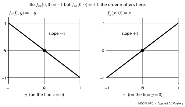
because \({f(0, y) = 0}\). At \({y = 0}\) the same holds, since \({f(h, 0) = 0}\). In the same way \({f_y(x, 0) = x}\) along the \(x\)-axis.
M05.5.1-F5
Peano’s function. The slope in \(x\), measured up the \(y\)-axis, falls with slope \(-1\); the slope in \(y\), measured along the \(x\)-axis, rises with slope \(+1\). The two mixed partial derivatives at the origin differ.
Differentiate once more: \({f_{xy}(0, 0) = \tfrac{d}{dy}(-y) = -1}\) but \({f_{yx}(0, 0) = \tfrac{d}{dx}(x) = 1}\). No contradiction: away from the origin both mixed partial derivatives equal
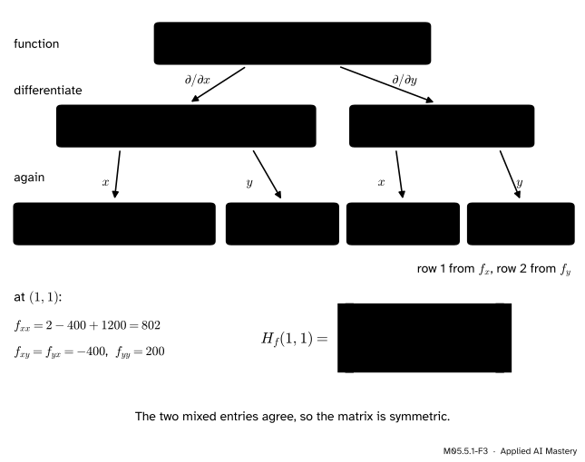
Along \(y\) only the last term of \(f_x\) depends on \(y\), so \({f_{xy} = -400x}\). From \(f_y\): \({f_{yx} = 200 \cdot (-2x) = -400x}\) and \({f_{yy} = 200}\). The mixed pair agree, as Schwarz’s theorem promises for a polynomial.
M05.5.1-F3
The worked example as a trace: differentiate once, differentiate each result again along each input, then evaluate at \({(1, 1)}\).
A second point. At the origin the same formulas give \({f_{xx} = 2}\), \({f_{xy} = 0}\) and \({f_{yy} = 200}\). Unlike the bowl and the running loss, whose Hessians are the same everywhere, Rosenbrock’s Hessian changes from point to point, because the function is not a quadratic.
Code
From scratch: column \(j\) of the Hessian is the change of the gradient along input \(j\), measured by a central difference. That costs \({2n}\) gradient evaluations.
import numpy as npdef rosen(p): x, y = preturn (1- x) **2+100* (y - x **2) **2def rosen_grad(p): x, y = preturn np.array([-2* (1- x) -400* x * (y - x **2), 200* (y - x **2)])def hessian_from_gradient(grad, a, h=1e-5):"""Column j: (grad(a + h e_j) - grad(a - h e_j)) / 2h.""" a = np.asarray(a, dtype=float) n = a.size H = np.empty((n, n))for j inrange(n): e = np.zeros(n) e[j] = h H[:, j] = (grad(a + e) - grad(a - e)) / (2* h)return HH_fd = hessian_from_gradient(rosen_grad, [1.0, 1.0])print(np.round(H_fd, 4))print("asymmetry:", abs(H_fd[0, 1] - H_fd[1, 0]))loss_grad =lambda p: np.array([15* p[0] +5* p[1] -23.5, 5* p[0] +2* p[1] -8])print(np.round(hessian_from_gradient(loss_grad, [0.0, 0.0]), 6))
A finite-difference Hessian is symmetric only up to rounding, so the two mixed entries can differ in their last digits. Now the library. scipy.differentiate.hessian wants a function that takes an array whose first axis holds the inputs, and it returns an object whose ddf attribute is the Hessian.
from scipy.differentiate import hessianres = hessian(rosen, np.array([1.0, 1.0]))print(res.ddf)print("converged:", res.success.all())
[[ 802. -400.]
 [-400.  200.]]
converged: True
Finally, Peano’s function: differentiate in the two orders at the origin, with a tiny inner step inside a larger outer one.
def peano(x, y):return0.0if x ==0and y ==0else x * y * (x **2- y **2) / (x **2+ y **2)h, k =1e-7, 1e-3# inner step, outer stepfx =lambda x, y: (peano(x + h, y) - peano(x - h, y)) / (2* h)fy =lambda x, y: (peano(x, y + h) - peano(x, y - h)) / (2* h)f_xy = (fx(0, k) - fx(0, -k)) / (2* k) # first along x, then along yf_yx = (fy(k, 0) - fy(-k, 0)) / (2* k) # first along y, then along xprint(round(f_xy, 4), round(f_yx, 4))
-1.0 1.0
Explore
This module’s interactive, the curvature viewer, lives in lesson M05.5.2. Pick Rosenbrock there and drag the point from the origin towards \({(1, 1)}\): the Hessian in the read-out changes at every step, while for the running bowl and the saddle it never does.
Pitfalls
M05.5.1-F4
Wrong beside right. A quadratic model built from the diagonal entries alone has upright contour lines; with the off-diagonal 5 it lies exactly on the running loss.
“The curvature is just the two second derivatives along the axes.”
The diagonal entries describe the function along the coordinate axes only. The off-diagonal entries tilt the picture: without them the contour lines of the running loss would stand upright, as on the left of the figure, and the valley would point the wrong way. In a model with many weights most of the interesting curvature is off the diagonal, between weights that work together.
“The mixed partial derivatives are always equal, so I never need to check.”
They are equal when they are continuous, which covers every polynomial, the sigmoid, \(\tanh\) and the usual losses. Peano’s function shows that the hypothesis is not decoration. Networks with ReLU units have kinks where second derivatives do not exist at all, so a Hessian there is a statement about the smooth pieces on either side.
“numpy.linalg.eigvalsh will tell me the eigenvalues of my numerical Hessian.”
It will, but it reads only the lower triangle of the matrix you pass. A finite-difference Hessian that is slightly asymmetric, or a matrix with a bug in its upper half, is silently replaced by a symmetric one. Symmetrise first, with \({(\mat{H} + \mat{H}\T)/2}\), and check that the asymmetry you removed was small.
Check yourself
Recall
1. What is in row \(i\), column \(j\) of the Hessian of \({f : \R^n \to \R}\)?
Show answer
The second partial derivative \({\frac{\partial}{\partial x_j}\big(\pd{f}{x_i}\big)}\): differentiate along \(x_i\), then along \(x_j\).
2. The Hessian is the Jacobian of which map, and what does \({\mat{H}\vect{h}}\) approximate?
Show answer
Of the gradient map \({\vect{x} \mapsto \nabla f(\vect{x})}\). \({\mat{H}\vect{h}}\) approximates the change of the gradient, \({\nabla f(\vect{a} + \vect{h}) - \nabla f(\vect{a})}\).
3. Under what condition is the Hessian symmetric, and what is the theorem called?
Show answer
When the second partial derivatives are continuous near the point: Schwarz’s theorem, also called Clairaut’s theorem.
4. What are the Hessians of the running bowl and of the running loss?
Show answer
\({\begin{bmatrix} 2 & 0 \\ 0 & 4 \end{bmatrix}}\) and \({\begin{bmatrix} 15 & 5 \\ 5 & 2 \end{bmatrix}}\), the same at every point because both functions are quadratic.
5. In the running loss, which term produces the off-diagonal 5, and what does that entry mean?
Show answer
The term \({5wb}\). The entry says how fast the slope in \(w\) changes when \(b\) moves, and equally how fast the slope in \(b\) changes when \(w\) moves.
Exercises
1.★ Find the Hessian of \({f(x, y) = x^3 y + 2y^2 - xy}\) at \({(1, 2)}\).
Show solution
\({f_x = 3x^2 y - y}\) and \({f_y = x^3 + 4y - x}\). Then \({f_{xx} = 6xy}\), \({f_{xy} = 3x^2 - 1}\), \({f_{yx} = 3x^2 - 1}\) and \({f_{yy} = 4}\). At \({(1, 2)}\):
2.★★ Let \({\mat{A} = \begin{bmatrix} 1 & 2 \\ 0 & 3 \end{bmatrix}}\), which is not symmetric, and \({f(\vect{x}) = \vect{x}\T \mat{A} \vect{x}}\) for \({\vect{x} = (x, y)}\). Write \(f\) out, find its Hessian, and express it in terms of \(\mat{A}\).
Show solution
\({\vect{x}\T \mat{A} \vect{x} = x^2 + 2xy + 3y^2}\): the entry 2 above the diagonal and the 0 below it add up to the single coefficient of \({xy}\). Then \({f_{xx} = 2}\), \({f_{xy} = f_{yx} = 2}\) and \({f_{yy} = 6}\), so
The Hessian is symmetric even though \(\mat{A}\) is not; for a symmetric \(\mat{A}\) it is \({2\mat{A}}\).
3.★★★ For Rosenbrock’s function, compute the double difference \(\Delta\) of the proof at \({(1, 1)}\) with \({h = k = 0.1}\), and divide by \({hk}\). You get \(-420\), not \({f_{xy}(1, 1) = -400}\). Show that \({\Delta / (hk)}\) is the average of \(f_{xy}\) over the square \({[1, 1.1] \times [1, 1.1]}\), and use this to explain \(-420\) exactly.
So \(\Delta = 1.22 - 4.42 - 1 + 0 = -4.2\) and \({\Delta / 0.01} = -420\).
By the fundamental theorem of calculus along \(y\), \({f_x(x, b + k) - f_x(x, b)}\) is the integral of \({f_{xy}(x, y)}\) over \({y}\) from \(b\) to \({b + k}\). Integrating that along \(x\) from \(a\) to \({a + h}\) turns the left side into \(\Delta\), because \(f_x\) integrates back to \(f\). So \(\Delta\) is the double integral of \(f_{xy}\) over the square, and \({\Delta / (hk)}\) is its average there. Here \({f_{xy} = -400x}\), whose average over the square is \({-400 \times 1.05 = -420}\), since \(x\) averages 1.05. As the square shrinks the average tends to \({f_{xy}(1, 1) = -400}\).
Summary card
The Hessian is the rate of change of the gradient.
M05.5.1-F1
Columns: how the gradient moves.
Entries.\({\mat{H}_{ij} = \frac{\partial}{\partial x_j}\big(\pd{f}{x_i}\big)}\), an \({n \times n}\) matrix.
Symmetry. Continuous second partials give \({\mat{H} = \mat{H}\T}\) (Schwarz).
Running examples. Bowl \({\operatorname{diag}(2, 4)}\); loss \({[[15, 5], [5, 2]]}\); Rosenbrock at \({(1, 1)}\): \({[[802, -400], [-400, 200]]}\).
Sources and next steps
Sources. Each was opened and checked against this lesson on 15 November 2026.
Gilbert Strang and Edwin Herman, Calculus Volume 3, Section 4.3, Partial derivatives, OpenStax. Defines the higher-order partial derivatives with the subscript order used here (\({f_{xy}}\) is differentiated first in \(x\)) and states Theorem 4.5, the equality of mixed partial derivatives (Clairaut’s theorem), under continuity on an open disc.
Marc Peter Deisenroth, A. Aldo Faisal and Cheng Soon Ong, Mathematics for Machine Learning, Section 5.7. Equation (5.146) states that the mixed partials of a twice continuously differentiable function agree and (5.147) defines the symmetric Hessian.
Alan Edelman and Steven G. Johnson, Matrix Calculus for Machine Learning and Beyond, MIT course notes, Section 12.1: the Hessian as the Jacobian of \({\nabla f}\), and \({\mat{H}\,d\vect{x}}\) as the first-order change of the gradient.
Wikipedia, Symmetry of second derivatives: Schwarz’s theorem, the proof by the mean value theorem applied to a double difference, and Peano’s counterexample with mixed partials \(-1\) and \(1\) at the origin.
Next.M05.5.2 The second-order Taylor model puts the Hessian to work: value, gradient and Hessian together give the best quadratic approximation of a function near a point.