A loss takes every weight of a model at once and returns one number; softmax takes a list of scores and returns a list of probabilities. Learn to name the domain, codomain and output shape of any function of many inputs, and write it for a whole batch in NumPy.
M05.1.1L2 Intermediate25 minIn review (what this means)
The maths and code on this page are checked by automated tests on every change, but an independent reader has not signed it off yet. Spot a mistake or a confusing step? Tell us.
Name the domain, the codomain, the range and the output shape of a function from R^n to R^m.
Evaluate by hand the running loss, a linear model of three features and the logistic model built on it.
Compute softmax of three scores by hand and explain why its outputs add up to 1.
Write a function for one input, then vectorise it over a batch with NumPy, asserting every shape.
The question
A small classifier of handwritten digits takes 784 pixel values and returns ten probabilities, one per digit. With one hidden layer of 100 units it has 79,510 weights and biases, and its loss takes every one of them and returns a single number. Neither is a function of one variable, and neither can be drawn as a curve. What kind of object is each of them, what shape is its output, and how do we evaluate it on a thousand inputs at once?
Intuition
In M04.10 a function took two numbers and returned one, and we drew it as a contour map. Machine learning needs more freedom on both sides: many numbers in, and one number or many numbers out. Sorting functions by those two counts tells you at once what kind of picture each one can have.
M05.1.1-F1
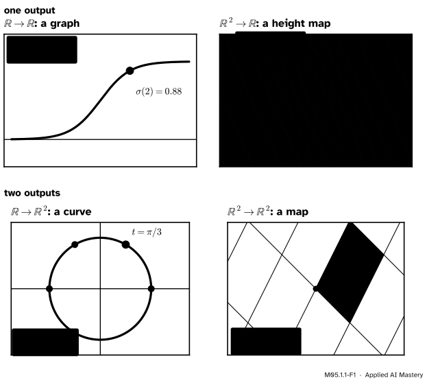
Four kinds of function, sorted by how many numbers go in and how many come out. One output can be drawn as a height; two outputs are a point that moves, as a curve or as a whole plane being warped.
Read the picture by its two counts. With one output, the function gives a height, and the picture is a graph or a height map. With several outputs, each input is sent to a point, so the picture shows where points go: one input traces a curve, two inputs warp a whole plane. A loss is always of the first kind. A layer of a network, which turns one list of numbers into another, is of the second.
Build it up
Step 1. A list of numbers in. Write the inputs as one vector, \({\vect{x} = (x_1, \dots, x_n)}\), a point of \(\R^n\). The running loss of M04.10 has \({n = 2}\) inputs, the slope and the intercept, and
So \({L(1, 0)} = {7.5 - 23.5 + 18.5} = {2.5}\) and \({L(1.4, 0.5) = 0.05}\).
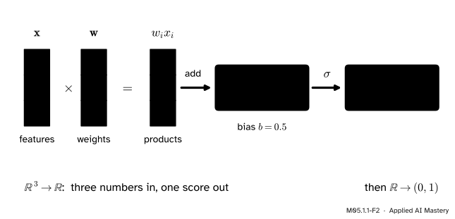
Step 2. One number out: a scalar field. A linear model with \(d\) features multiplies each feature by its weight and adds a bias: \({f(\vect{x}) = \vect{w}\T\vect{x} + b}\). Take \({d = 3}\), weights \({\vect{w} = (0.5, -1, 2)}\), \({b = 0.5}\) and the input \({\vect{x} = (2, 1, 1)}\). Then
Step 3. Compose with one more step. The logistic model feeds that score \(z\) into the sigmoid \({\sigma(z) = 1/(1 + e^{-z})}\), so \({p = \sigma(2.5) \approx 0.924}\). Three numbers went in, one probability came out.
M05.1.1-F2
A linear model of three features, then the sigmoid. Each step returns fewer numbers or the same number, never more: three features become one score, and the score becomes one probability.
Step 4. Many numbers out. Softmax turns a list of \(K\) scores into \(K\) probabilities. It exponentiates each score, so every entry becomes positive, then divides by the total, so the entries add up to 1:
With \({K = 3}\) it is a function from \(\R^3\) to \(\R^3\). The worked example below evaluates it.
Step 5. One number in, many out. A parametrised curve sends a time \(t\) to a point. The curve \({\vect{r}(t) = (\cos t, \sin t)}\) goes from \(\R\) to \(\R^2\) and traces the unit circle; at \({t = \pi/3}\) it is at \({(0.5, 0.866)}\).
The formal statement
NoteDefinition: a function of several variables
A function \({f : D \to \R^m}\) with domain\(D\), a set of points of \(\R^n\), assigns to each \({\vect{x}}\) in \(D\) exactly one output \({f(\vect{x})}\) in \(\R^m\), its codomain. The set of outputs that actually occur is the range.
When \({m = 1}\), \(f\) is a scalar field (or real-valued function of \(n\) variables).
When \({m > 1}\), \(f\) is vector-valued. Its \(m\) entries are scalar fields of their own, \({f(\vect{x}) = (f_1(\vect{x}), \dots, f_m(\vect{x}))}\), the components of \(f\).
Four facts follow from the definition, and later lessons lean on each.
The output has a shape. A scalar field returns one number. A vector-valued \(f\) returns a vector with \(m\) entries. In code these are NumPy shapes () and (m,), and the input has shape (n,). Keeping these straight is most of the work of matrix calculus (M05.7).
The domain can be smaller than \(\R^n\). The running program of this course, \({f(x_1, x_2) = \ln x_1 + x_1 x_2 - \sin x_2}\), needs \({x_1 > 0}\), because the logarithm does. Its domain is the half-plane to the right of the \(x_2\) axis. At \((2, 5)\),
The range can be much smaller than the codomain. The sigmoid has codomain \(\R\), but its range is the open interval from 0 to 1. Softmax has codomain \(\R^3\), but every output has positive entries that add up to 1: its range lies inside a triangle, a flat piece of a plane in \(\R^3\).
Only small cases can be drawn. The graph of a scalar field is the set of points \({(\vect{x}, f(\vect{x}))}\), which lives in \(\R^{n+1}\). For \({n = 2}\) that is a surface in space; for \({n = 3}\) it would need four dimensions. Lessons 2 and 3 of this module give two ways round that: level sets and slices.
Go deeper: why softmax ignores a shift of all its scores
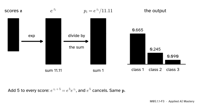
Add the same number \(c\) to every score. Each exponential gains the factor \(e^c\), since \({e^{z_i + c} = e^c e^{z_i}}\), and so does the total:
So softmax sends the whole line of inputs \({\vect{z} + c\,(1, 1, 1)}\) to one output: one of its three input directions is lost completely. That fits with what the range showed: the outputs keep only two degrees of freedom, because they must add up to 1, which puts them on a plane. Libraries use the lost direction: they subtract the largest score before exponentiating, so that \(e^{z_i}\) never overflows.
Worked example
Softmax of the scores \({\vect{z} = (2, 1, 0)}\).
Exponentiate.\({e^2 \approx 7.389}\), \({e^1 \approx 2.718}\) and \({e^0 = 1}\).
The three add up to 1, as they must, and the largest score gets the largest probability. The output is not just the scores rescaled: the scores are evenly spaced, but each probability is \({e \approx 2.718}\) times the next.
M05.1.1-F3
Softmax step by step. The output is three positive numbers that add up to 1, and adding the same number to every score leaves it unchanged.
A curve, then a scalar field along it. Feed the circle \({\vect{r}(t) = (\cos t, \sin t)}\) into the running bowl \({f(x, y) = x^2 + 2y^2}\). The composite takes one number to one number:
\[
\begin{aligned}
f(\vect{r}(t)) &= \cos^2 t + 2\sin^2 t \\
&= 1 + \sin^2 t ,
\end{aligned}
\]
using \({\cos^2 t + \sin^2 t = 1}\). At \({t = \pi/4}\) it is \({1 + 1/2 = 1.5}\). Walking once round the circle, the height rises and falls twice, between 1 on the \(x\) axis and 2 on the \(y\) axis. Restricting a function of many inputs to a curve or a line is how lesson 3 draws it.
Code
First each function for a single input, written plainly, with its output shape asserted.
import numpy as npdef loss(w, b):"""The running loss of M04.10: two numbers in, one out."""return7.5* w**2+5* w * b + b**2-23.5* w -8* b +18.5w = np.array([0.5, -1.0, 2.0])b =0.5def linear(x):"""A linear model of three features: R^3 -> R."""return w @ x + bdef logistic(x):return1/ (1+ np.exp(-linear(x)))def softmax(z):"""R^K -> R^K. Subtracting the largest score changes nothing and avoids overflow.""" e = np.exp(z - np.max(z))return e / e.sum()x = np.array([2.0, 1.0, 1.0])p = softmax(np.array([2.0, 1.0, 0.0]))print(loss(1, 0), round(loss(1.4, 0.5), 4))print(linear(x), round(float(logistic(x)), 3))print(p.round(3), p.shape)
2.5 0.05
2.5 0.924
[0.665 0.245 0.09 ] (3,)
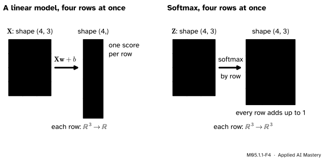
Now a batch: four inputs stacked as the rows of a matrix \(\mat{X}\) of shape (4, 3). The product X @ w takes the dot product of every row with \(\vect{w}\) at once, and adding the number b adds it to every entry. For softmax, each row is one list of scores, so the maximum and the sum must be taken along each row (axis=1), with keepdims=True keeping a column that lines up with the rows.
A batch is a stack of inputs, one per row. A scalar field gives one number per row, shape (4,); softmax gives one row of probabilities per row, shape (4, 3).
SciPy has both functions ready-made. scipy.special.expit is the sigmoid, applied entry by entry. scipy.special.softmax normalises over the whole array unless it is given an axis, so a batch needs axis=1.
from scipy.special import expit, softmax as sp_softmaxprint(np.allclose(expit(scores), probs), np.allclose(sp_softmax(X, axis=1), P))print("no axis, row sums:", sp_softmax(X).sum(axis=1).round(3))
True True
no axis, row sums: [0.413 0.097 0.358 0.132]
Explore
This module’s interactive, the level-set explorer, lives in lesson M05.1.3. It draws four of this lesson’s scalar fields, among them the running loss and the logistic model, as contour maps.
Pitfalls
M05.1.1-F5
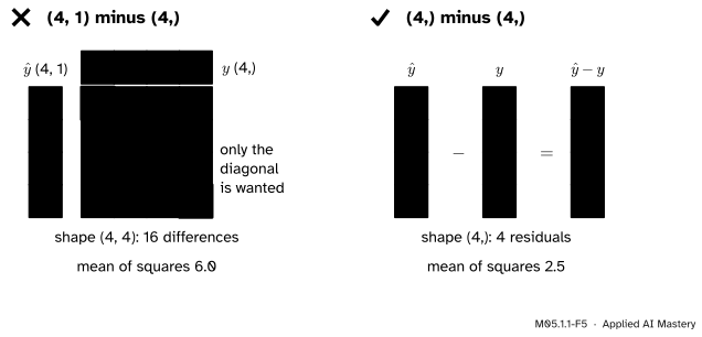
Wrong beside right. The predictions of the line \({\hat{y} = x}\), the point \({(w, b) = (1, 0)}\), on the four points of the running loss, as a column of shape (4, 1), minus the targets of shape (4,), broadcast to a table of all 16 differences. The mean of their squares is 6.0, not the loss 2.5.
“NumPy will complain if the shapes are wrong.”
Often it will not. NumPy compares shapes from the last axis backwards, and a length of 1 is stretched to match. So a column of four predictions minus a flat array of four targets quietly becomes a (4, 4) table, and its mean is a number that looks plausible. The cure is to assert the shape of every intermediate result, as the code above does, and to keep vectors flat, shape (n,), unless a column is really meant.
“Softmax works on whatever array I give it.”
It works on one list of scores. Given a whole batch without an axis, scipy.special.softmax divides by the total of all twelve exponentials, so the probabilities of each example no longer add up to 1. Name the axis that runs over the classes.
“A function from \(\R^3\) to \(\R^3\) can reach any point of \(\R^3\).”
The codomain is only where outputs are allowed to live. Softmax never returns a negative entry or a list whose total is not 1, so most of \(\R^3\) is out of its reach. When a later lesson asks how an output changes, it changes only within the range.
Check yourself
Recall
1. What are \(n\) and \(m\) for the running loss \({L(w, b)}\), for softmax of three scores, and for the curve \({(\cos t, \sin t)}\)?
Show answer
The loss goes from \(\R^2\) to \(\R\), so \({n = 2}\), \({m = 1}\). Softmax of three scores goes from \(\R^3\) to \(\R^3\): \({n = m = 3}\). The curve goes from \(\R\) to \(\R^2\): \({n = 1}\), \({m = 2}\).
2. What is the difference between the codomain and the range of a function?
Show answer
The codomain is the space the outputs are said to live in, such as \(\R^m\). The range is the set of outputs that actually occur. The sigmoid has codomain \(\R\) and range the open interval from 0 to 1.
3. What is a scalar field, and what are the components of a vector-valued function?
Show answer
A scalar field is a function with one number as output (\({m = 1}\)). A vector-valued \(f\) has \(m\) outputs, and each output, \({f_i(\vect{x})}\), is a scalar field: a component of \(f\).
4. A batch \(\mat{X}\) has shape (32, 5) and \(\vect{w}\) has shape (5,). What is the shape of X @ w + b, for a number b?
Show answer
(32,): one score for each of the 32 rows.
5. Why do the outputs of softmax always add up to 1?
Show answer
Each output is \({e^{z_i}}\) divided by the sum of all the \({e^{z_k}}\), so the outputs add up to that sum divided by itself.
Exercises
1.★ With \({\vect{w} = (0.5, -1, 2)}\) and \({b = 0.5}\), evaluate the linear model and the logistic model at \({\vect{x} = (1, 2, 0)}\).
2.★★ Compute softmax of \({(0, 0, \ln 2)}\) exactly, and then of \({(5, 5, 5 + \ln 2)}\) without new arithmetic.
Show solution
The exponentials are 1, 1 and \({e^{\ln 2} = 2}\), with total 4, so the output is \({(1/4, 1/4, 1/2)}\). The second list is the first plus 5 in every entry, so by the shift rule its softmax is the same, \({(0.25, 0.25, 0.5)}\).
3.★★★ A batch of \(N\) inputs with \(d\) features is stored as X of shape (N, d), and a layer has a weight matrix W of shape (d, k) and a bias c of shape (k,). Give the shape of X @ W + c, say which function from \(\R^d\) to \(\R^k\) it applies to each row, and explain why the broadcast of c is the one you want.
Show solution
X @ W has shape (N, k): row \(i\) is \({\vect{x}_i\T \mat{W}}\), the \(k\) outputs for example \(i\). So each row goes through the map \({\vect{x} \mapsto \mat{W}\T\vect{x} + \vect{c}}\) from \(\R^d\) to \(\R^k\), written with columns. Adding c of shape (k,) to an array of shape (N, k): aligning from the right, \(k\) matches \(k\), and the missing first axis is stretched to \(N\), so the same bias is added to every row, which is what the layer means. Had c been a column of shape (N, 1), it would have added a different number to each example instead.
Summary card
Count the inputs and the outputs: \(\R^n \to \R\) is a height, \(\R^n \to \R^m\) moves points.
M05.1.1-F1
Four kinds of function.
Function:\({f : D \to \R^m}\) with \(D\) in \(\R^n\); components \({f_1, \dots, f_m}\).
Shapes: input (n,), output () or (m,); a batch (N, n) gives (N,) or (N, m).
Linear model:\({\vect{w}\T\vect{x} + b}\), from \(\R^d\) to \(\R\).
Softmax:\({e^{z_i} / \sum_k e^{z_k}}\), positive entries adding up to 1.
Habit: assert every shape; broadcasting does not complain.
Sources and next steps
Sources. Each was opened and checked against this lesson on 15 November 2026.
Gilbert Strang and Edwin Herman, Calculus Volume 3 (OpenStax), Section 4.1: a function of two variables assigns one real number to each pair in a domain \(D\), the range is the set of values it produces, and the section goes on to functions of three variables.
Marc Peter Deisenroth, A. Aldo Faisal and Cheng Soon Ong, Mathematics for Machine Learning, Section 5.3: a vector-valued function from \(\R^n\) to \(\R^m\) is viewed as the vector of its \(m\) real-valued component functions, equation (5.54).
NumPy 2.5 user guide, Broadcasting: shapes are compared from the trailing dimension leftwards, two dimensions are compatible when they are equal or one of them is 1, and an array of shape (4, 1) plus one of shape (3,) gives shape (4, 3).
SciPy reference, scipy.special.softmax (with the default axis=None the softmax is computed over the entire array) and scipy.special.expit (the logistic sigmoid \({1/(1 + e^{-x})}\), applied element-wise).
Next.M05.1.2 Level sets draws a scalar field of any number of inputs by the sets where it takes one value.