Minimum, maximum or saddle: the second-derivative test
Where the gradient is zero the Taylor model is pure curvature, so the signs of the Hessian’s eigenvalues decide: a minimum, a maximum or a saddle. Prove the test, apply it to the running loss and a cubic, and see the monkey saddle where it says nothing.
M05.5.3L2 Intermediate25 minIn review (what this means)
The maths and code on this page are checked by automated tests on every change, but an independent reader has not signed it off yet. Spot a mistake or a confusing step? Tell us.
Explain why, at a critical point, the signs of the Hessian’s eigenvalues decide between a minimum, a maximum and a saddle.
Prove the second-derivative test for a positive definite Hessian and for an indefinite one.
Apply the eigenvalue test and the two-variable test with f_xx and det H to classify critical points by hand.
Recognise the semidefinite cases where the test is silent, with x^4 + y^4, the monkey saddle, x^2 + y^4 and x^2 - y^4.
Classify critical points in code with numpy.linalg.eigvalsh and a tolerance.
The question
Gradient descent stops where the gradient is zero. But the gradient is also zero on top of a hill and in the middle of a saddle, where the ground rises one way and falls another. Given a point where \({\nabla f = \vect{0}}\), how do you tell which of the three it is, and when is it impossible to tell from second derivatives alone? For the losses of large networks the question is not idle: most of their flat points turn out to be saddles.
From the last lesson
1. For the slice \({g(t) = f(\vect{a} + t\vect{h})}\), what are \({g'(0)}\) and \({g''(0)}\)?
Show answer
\({g'(0) = \nabla f(\vect{a})\T \vect{h}}\) and \({g''(0) = \vect{h}\T \mat{H}_f(\vect{a})\vect{h}}\).
2. Between which two numbers must the curvature \({\vect{u}\T \mat{H}\vect{u}}\) lie for a unit \(\vect{u}\)?
Show answer
Between the smallest and the largest eigenvalue of \(\mat{H}\).
Intuition
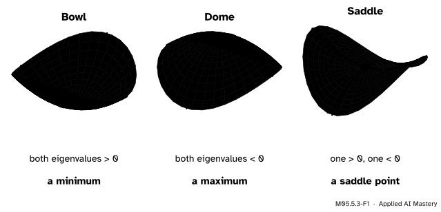
At a critical point, a point where \({\nabla f(\vect{a}) = \vect{0}}\), the gradient term of the Taylor model vanishes and only the curvature term is left. Near \(\vect{a}\), the function is its value plus a pure quadratic, and a pure quadratic has only three basic shapes.
M05.5.3-F1
The quadratic model at a critical point. Positive curvature in every direction makes a bowl, negative in every direction a dome, and mixed signs a saddle.
Which shape you get depends only on the signs of the Hessian’s eigenvalues. They are the curvatures along the two perpendicular eigen-directions, and every other direction’s curvature is an average of them (M05.5.2). If both are positive every direction curves up; if both are negative every direction curves down; if one of each, some directions go up and some go down.
Build it up
Step 1. Drop the gradient term. At a critical point the model of M05.5.2 reads
Step 2. Turn the axes. Write the step in the Hessian’s orthonormal eigenvectors, \({\vect{h} = s\,\vect{q}_1 + t\,\vect{q}_2}\). Because \({\mat{H}\vect{q}_i = \lambda_i \vect{q}_i}\) and the \(\vect{q}_i\) are perpendicular unit vectors, the cross terms drop out:
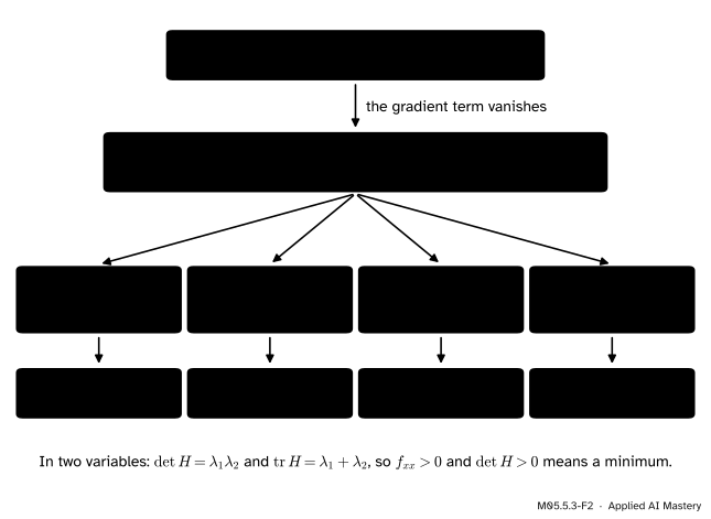
Step 3. Read the signs. A sum of squares with positive weights is positive for every step: a minimum. Negative weights make it negative: a maximum. Weights of opposite signs make it positive along one axis and negative along the other: a saddle. A zero weight leaves one direction where the model is flat, and there the cubic and higher terms, which the model ignores, decide.
M05.5.3-F2
From a critical point to a verdict. Everything rests on the signs of the eigenvalues.
Step 4. Two variables without eigenvalues. For a \({2 \times 2}\) Hessian \({\det \mat{H} = \lambda_1 \lambda_2}\). If \({\det \mat{H} > 0}\) the eigenvalues share a sign, and \(f_{xx}\), the curvature along \({(1, 0)}\), lies between them and so has that sign too. If \({\det \mat{H} < 0}\) they have opposite signs. This is the test \({a > 0}\), \({ac - b^2 > 0}\) of M03.4.2 for a positive definite matrix.
The formal statement
NoteTheorem: the second-derivative test
Let \(f\) have continuous second partial derivatives near \(\vect{a}\), with \({\nabla f(\vect{a}) = \vect{0}}\), and let \({\mat{H} = \mat{H}_f(\vect{a})}\).
If \(\mat{H}\) is positive definite (every eigenvalue \({> 0}\)), \(\vect{a}\) is a strict local minimum.
If \(\mat{H}\) is negative definite (every eigenvalue \({< 0}\)), \(\vect{a}\) is a strict local maximum.
If \(\mat{H}\) is indefinite (eigenvalues of both signs), \(\vect{a}\) is a saddle point: neither a local minimum nor a local maximum.
Otherwise some eigenvalue is 0 and the rest share a sign, and the test is silent.
In two variables, with \({D = f_{xx} f_{yy} - f_{xy}^2 = \det \mat{H}}\): \({D > 0}\) and \({f_{xx} > 0}\) give a minimum, \({D > 0}\) and \({f_{xx} < 0}\) a maximum, \({D < 0}\) a saddle, and \({D = 0}\) says nothing.
Go deeper: proof of parts 1 and 3
Part 1. Let \({\lambda_{\min} > 0}\) be the smallest eigenvalue. By the Rayleigh bound of M05.5.2, \({\vect{h}\T \mat{H}\vect{h} \ge \lambda_{\min} \norm{\vect{h}}^2}\) for every \(\vect{h}\). By the Taylor theorem of M05.5.2,
with \({r(\vect{h}) / \norm{\vect{h}}^2 \to 0}\). So there is a radius \(\delta\) such that \({\abs{r(\vect{h})} \le \tfrac14 \lambda_{\min} \norm{\vect{h}}^2}\) whenever \({\norm{\vect{h}} < \delta}\). For those steps, with \({\vect{h} \neq \vect{0}}\),
Every nearby point is higher: a strict local minimum. Part 2 is part 1 applied to \(-f\).
Part 3. Let \(\vect{q}_+\) be a unit eigenvector with eigenvalue \({\lambda_+ > 0}\) and \(\vect{q}_-\) one with \({\lambda_- < 0}\). The slice \({g(t) = f(\vect{a} + t\vect{q}_+)}\) has \({g'(0) = 0}\) and \({g''(0) = \lambda_+ > 0}\), so by the one-variable second-derivative test (M04.4) it has a strict local minimum at 0: points along \(\vect{q}_+\) arbitrarily close to \(\vect{a}\) are higher. Along \(\vect{q}_-\) the same argument finds points that are lower. So \(\vect{a}\) is neither. \(\square\)
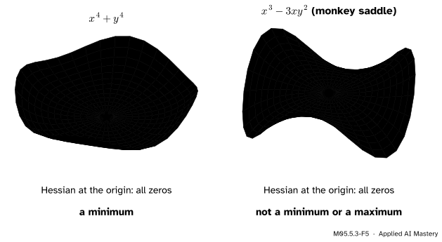
Why part 4 must be silent. When an eigenvalue is 0 the model is flat along its eigenvector, and the cubic or quartic terms decide. Four functions show that anything can happen. The Hessians of \({x^2 + y^4}\) and \({x^2 - y^4}\) at the origin are both \({\operatorname{diag}(2, 0)}\), yet the first has a minimum there and the second a saddle, since \({-y^4}\) falls along the \(y\)-axis. The Hessians of \({x^4 + y^4}\) and of the monkey saddle\({x^3 - 3xy^2}\) are both zero at the origin, yet the first is a minimum and the second rises and falls three times around it: along the \(x\)-axis it is \({x^3}\), which takes both signs.
M05.5.3-F5
Two functions whose Hessians at the origin are both zero. One is a minimum and one is not, so the Hessian alone cannot decide.
Worked example
The running loss. Lesson M04.10.4 found its one critical point, \({(1.4, 0.5)}\). The Hessian \({\begin{bmatrix} 15 & 5 \\ 5 & 2 \end{bmatrix}}\) has \({f_{xx} = 15 > 0}\) and \({D = 30 - 25 = 5 > 0}\), so it is a minimum; its eigenvalues \({(17 \pm \sqrt{269})/2 \approx 16.70}\) and \({0.299}\) are both positive. Because \(L\) is a quadratic its Taylor model is exact: with \({\vect{w}^* = (1.4, 0.5)}\),
so the minimum is the lowest point of the whole plane.
The saddle\({x^2 - y^2}\). The gradient \({(2x, -2y)}\) vanishes only at the origin, where \({\mat{H} = \operatorname{diag}(2, -2)}\) and \({D = -4 < 0}\): a saddle.
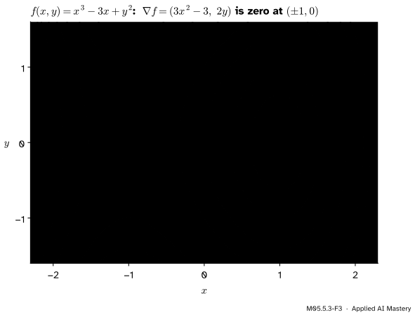
The cubic\({f(x, y) = x^3 - 3x + y^2}\).
Critical points.\({\nabla f = (3x^2 - 3,\; 2y)}\). The second entry is zero only for \({y = 0}\), the first for \({x^2 = 1}\). So there are two: \({(1, 0)}\) and \({(-1, 0)}\).
At \({(1, 0)}\).\({\mat{H} = \operatorname{diag}(6, 2)}\): both eigenvalues positive, a strict local minimum, with \({f(1, 0) = 1 - 3 = -2}\).
At \({(-1, 0)}\).\({\mat{H} = \operatorname{diag}(-6, 2)}\): opposite signs, a saddle, with \({f(-1, 0) = -1 + 3 = 2}\). Along \(x\) the point is the top of a hill, along \(y\) the bottom of a valley.
M05.5.3-F3
The cubic’s two critical points. Around the minimum the contour lines are ovals; at the saddle the level through it crosses itself.
The minimum at \({(1, 0)}\) is only local: along the \(x\)-axis \({f(x, 0) = x^3 - 3x}\) falls without bound as \(x\) runs to \({-\infty}\). The second-derivative test is a statement about a neighbourhood.
Code
A classifier from scratch. Eigenvalues come from numpy.linalg.eigvalsh; a tolerance decides what counts as zero, because a Hessian computed in floating point is never exactly singular.
import numpy as npdef classify(H, tol=1e-9): lam = np.linalg.eigvalsh((H + H.T) /2) scale =max(1.0, np.abs(lam).max())if np.any(np.abs(lam) <= tol * scale):return"saddle"if lam.min() <-tol * scale and lam.max() > tol * scale else"test silent"if lam.min() >0:return"minimum"if lam.max() <0:return"maximum"return"saddle"cases = {"running loss at (1.4, 0.5)": np.array([[15.0, 5.0], [5.0, 2.0]]),"x^2 - y^2 at (0, 0)": np.diag([2.0, -2.0]),"cubic at (1, 0)": np.diag([6.0, 2.0]),"cubic at (-1, 0)": np.diag([-6.0, 2.0]),"x^2 + 3xy + y^2 at (0, 0)": np.array([[2.0, 3.0], [3.0, 2.0]]),"x^2 + y^4 at (0, 0)": np.diag([2.0, 0.0]),"monkey saddle at (0, 0)": np.zeros((2, 2)),}verdicts = {name: classify(H) for name, H in cases.items()}for name, verdict in verdicts.items():print(f"{name:28s}{verdict}")
running loss at (1.4, 0.5)   minimum
x^2 - y^2 at (0, 0)          saddle
cubic at (1, 0)              minimum
cubic at (-1, 0)             saddle
x^2 + 3xy + y^2 at (0, 0)    saddle
x^2 + y^4 at (0, 0)          test silent
monkey saddle at (0, 0)      test silent
A preview of many dimensions. At a critical point of a loss with \(n\) weights, a minimum needs all \(n\) curvatures to be positive. As a rough model, draw random symmetric matrices and count how often every eigenvalue is positive.
rng = np.random.default_rng(0)share = {}for n in (1, 2, 3, 4, 6): A = rng.normal(size=(20000, n, n)) S = (A + np.transpose(A, (0, 2, 1))) /2# 20000 random symmetric matrices share[n] = (np.linalg.eigvalsh(S) >0).all(axis=1).mean()print({n: round(float(p), 4) for n, p in share.items()})
About half for one weight, about one in seven for two, a few in a thousand for four, and none of the 20,000 for six. Real losses are not random matrices, but the trend is the reason why saddles, not poor minima, dominate the flat points of large networks (M08.11).
Frontier note: saddle points in deep learning
Dauphin and co-authors argued in 2014, drawing on statistical physics, random-matrix theory, neural-network theory and experiments, that in high-dimensional problems the main difficulty is the proliferation of saddle points, not of poor local minima. Saddles are surrounded by plateaus of high error that slow learning and can look like local minima. They proposed a second-order method, the saddle-free Newton method, designed to escape them quickly. Course M08.11 takes this up.
Explore
The curvature viewer in lesson M05.5.2 applies this test. Choose each surface and press To the critical point: the bowl and Rosenbrock give a minimum, the saddle a saddle, and the monkey saddle a Hessian of zeros, where the read-out says that the test is silent.
Pitfalls
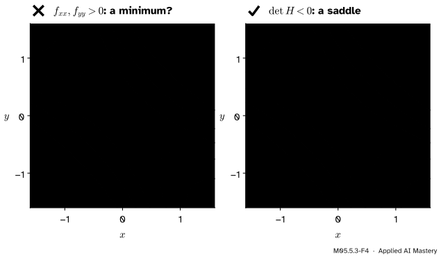
M05.5.3-F4
Wrong beside right for \({x^2 + 3xy + y^2}\). Both axis slices rise, yet along \({(1, -1)}\) the function falls: its Hessian \({[[2, 3], [3, 2]]}\) has eigenvalues 5 and \(-1\).
“Both second derivatives along the axes are positive, so it is a minimum.”
The axes are only two of the directions. For \({x^2 + 3xy + y^2}\), \({f_{xx} = f_{yy} = 2 > 0}\), but \({f(t, -t) = t^2 - 3t^2 + t^2 = -t^2}\) falls. The determinant \({4 - 9 = -5}\) catches it. Always use the whole Hessian: the eigenvalues, or \({f_{xx}}\) together with \({\det \mat{H}}\).
“The Hessian is zero, so the point is flat and therefore a minimum (or a saddle).”
A zero or singular Hessian means only that the test is silent. \({x^4 + y^4}\) has a minimum, the monkey saddle does not, and \({-x^4 - y^4}\) has a maximum, all with the same zero Hessian. Look at higher terms, or at the function along lines through the point.
“A strict local minimum is the lowest point.”
Only nearby. The cubic’s minimum at \({(1, 0)}\) has height \(-2\), yet \({f(-3, 0) = -18}\). A loss whose Hessian is positive semidefinite everywhere, like the running loss, is different: there every local minimum is global, the subject of convexity in M08.2.
Check yourself
Recall
1. What does the second-order Taylor model reduce to at a critical point?
Show answer
\({f(\vect{a} + \vect{h}) - f(\vect{a}) \approx \tfrac12 \vect{h}\T \mat{H}\vect{h}}\): the gradient term is gone.
2. State the verdict for each sign pattern of the eigenvalues of \(\mat{H}\) at a critical point.
Show answer
All positive: a strict local minimum. All negative: a strict local maximum. Both signs: a saddle. Some zero and the rest of one sign: the test is silent.
3. State the two-variable test using \({D = f_{xx} f_{yy} - f_{xy}^2}\).
Show answer
\({D > 0}\) and \({f_{xx} > 0}\): minimum. \({D > 0}\) and \({f_{xx} < 0}\): maximum. \({D < 0}\): saddle. \({D = 0}\): no conclusion.
4. Why is the test silent at the origin for the monkey saddle, and what is the point?
Show answer
Its Hessian there is the zero matrix. The point is neither a minimum nor a maximum, since along the \(x\)-axis the function is \({x^3}\), which takes both signs.
5. Classify the critical points of \({x^3 - 3x + y^2}\).
Show answer
\({(1, 0)}\), with Hessian \({\operatorname{diag}(6, 2)}\), is a strict local minimum; \({(-1, 0)}\), with \({\operatorname{diag}(-6, 2)}\), is a saddle.
Exercises
1.★ Find and classify the critical points of \({f(x, y) = x^2 + xy + y^2 - 3x}\).
Show solution
\({\nabla f = (2x + y - 3,\; x + 2y)}\). The second entry gives \({x = -2y}\); then \({-4y + y - 3 = 0}\), so \({y = -1}\) and \({x = 2}\). The Hessian \({\begin{bmatrix} 2 & 1 \\ 1 & 2 \end{bmatrix}}\) has \({f_{xx} = 2 > 0}\) and \({D = 4 - 1 = 3 > 0}\): a minimum, with \({f(2, -1) = 4 - 2 + 1 - 6 = -3}\).
2.★★ Find and classify the critical points of \({f(x, y) = x^3 + y^3 - 3xy}\).
Show solution
\({\nabla f = (3x^2 - 3y,\; 3y^2 - 3x)}\). The first entry gives \({y = x^2}\); the second then gives \({x^4 = x}\), so \({x = 0}\) or \({x = 1}\). The critical points are \({(0, 0)}\) and \({(1, 1)}\). The Hessian is \({\begin{bmatrix} 6x & -3 \\ -3 & 6y \end{bmatrix}}\).
At \({(0, 0)}\): \({D = 0 - 9 = -9 < 0}\), a saddle.
At \({(1, 1)}\): \({f_{xx} = 6 > 0}\) and \({D = 36 - 9 = 27 > 0}\), a minimum, with \({f(1, 1) = 1 + 1 - 3 = -1}\).
3.★★★ Prove the second-order necessary condition: if \(f\) has continuous second partial derivatives and a local minimum at \(\vect{a}\), then \({\mat{H}_f(\vect{a})}\) is positive semidefinite. Why does this not contradict the silence of the test?
Show solution
A local minimum in the interior has \({\nabla f(\vect{a}) = \vect{0}}\) (M04.10.4). Suppose some unit \(\vect{u}\) had \({\vect{u}\T \mat{H}\vect{u} < 0}\). The slice \({g(t) = f(\vect{a} + t\vect{u})}\) has \({g'(0) = \nabla f(\vect{a})\T \vect{u} = 0}\) and \({g''(0) = \vect{u}\T \mat{H}\vect{u} < 0}\), so by the one-variable test \(g\) has a strict local maximum at 0: there are points \({\vect{a} + t\vect{u}}\), as close to \(\vect{a}\) as we like, with \({f < f(\vect{a})}\). That contradicts the local minimum. So \({\vect{u}\T \mat{H}\vect{u} \ge 0}\) for every \(\vect{u}\).
The condition runs one way only. A positive semidefinite Hessian is necessary for a minimum but not sufficient: \({x^2 - y^4}\) has Hessian \({\operatorname{diag}(2, 0)}\) at the origin and no minimum there. That is exactly the case where the test is silent.
Summary card
At a critical point, the eigenvalues’ signs decide.
M05.5.3-F1
Bowl, dome or saddle.
Model. In eigen-coordinates the change is about \({\tfrac12 \lambda_1 s^2} + {\tfrac12 \lambda_2 t^2}\).
Test. All \({\lambda > 0}\): minimum. All \({\lambda < 0}\): maximum. Mixed: saddle. A zero: silent.
Two variables.\({D = f_{xx} f_{yy} - f_{xy}^2}\) with the sign of \(f_{xx}\).
Silent examples.\({x^4 + y^4}\) (minimum), the monkey saddle (neither).
Sources and next steps
Sources. Each was opened and checked against this lesson on 15 November 2026.
Gilbert Strang and Edwin Herman, Calculus Volume 3, Section 4.7, Maxima/minima problems, OpenStax. The definitions of a critical point and a saddle point, and Theorem 4.17, the second derivative test with \({D = f_{xx} f_{yy} - f_{xy}^2}\), including the inconclusive case \({D = 0}\).
Alan Edelman and Steven G. Johnson, Matrix Calculus for Machine Learning and Beyond, Section 12.4.3: a positive definite second derivative at a critical point gives a minimum, a negative definite one a maximum, an indefinite one a saddle; with zero eigenvalues higher derivatives decide; and the \({2 \times 2}\) check by \({\det \mat{H}}\) and \({\operatorname{tr}\mat{H}}\).
Next.M05.5.4 Curvature of a loss computes the Hessians of the losses that models are trained on, and uses their curvature to take a Newton step and to set a learning rate.