Draw a 2-2-1 network for XOR as a computational graph, run the forward pass by hand, then the backward pass of reverse mode: the output adjoint p - y, through the weights, through tanh’, into every weight. Backpropagation is nothing more.
M05.9.1L2 Intermediate25 minIn review (what this means)
The maths and code on this page are checked by automated tests on every change, but an independent reader has not signed it off yet. Spot a mistake or a confusing step? Tell us.
Write a 2-2-1 network with tanh hidden units, a sigmoid output and the log loss as a computational graph, and run its forward pass by hand.
Derive that the adjoint of the output score is p - y for a sigmoid output with the log loss.
Pass adjoints backward through a dense layer and through tanh, and read off every weight gradient for one example.
Check a hand-computed backward pass against a reverse-mode Var class and against central differences.
The question
A tiny network has to learn XOR: output 1 when exactly one of two inputs is 1. With its starting weights it looks at the input \({(0, 1)}\) and says the chance of a 1 is only 0.121. It has nine parameters, weights and biases. Which way should each one move, and by how much does each matter? Lesson M05.8.3 gave a method that answers this for every weight in one backward sweep. Is “backpropagation” anything more than that method?
Intuition
A neural network is a program. Run it on one example and it leaves a trace: inputs, hidden values, an output, a loss. So it is a computational graph, and reverse mode applies unchanged: values flow forward, adjoints flow back from the loss, and each weight collects its adjoint on the way.
M05.9.1-F1
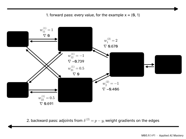
The running network on the example \({\vect{x} = (0, 1)}\). Forward values (vermillion) fill the nodes from left to right; adjoints \(\delta\) (green) come back from the loss; every weight’s gradient is its edge’s adjoint times the value that flowed along the edge.
Read the picture from right to left. The loss of 2.114 is large because the network said 0.121 where the label is 1. The output score \(z^{(2)}\) should go up, so its adjoint is negative: raising \(z^{(2)}\) lowers the loss. That adjoint is shared out to the two hidden units in proportion to the weights they speak through, damped by the slope of tanh at each unit, and finally handed to the weights of the first layer. The weights from \(x_1\) get nothing, because \(x_1 = 0\) in this example: nudging them changes nothing.
This is backpropagation: reverse-mode automatic differentiation applied to a network’s loss as a function of its weights. Nothing about it is special to networks except the shape of the graph.
Build it up
Step 1. The network. The running network of this course (M05 conventions) has two inputs, two tanh hidden units and one sigmoid output:
The loss of one example with label \(y\) is the log loss \({\ell} = {-y \ln p - (1 - y)\ln(1 - p)}\), and for the whole XOR batch the mean of the four. The starting weights, fixed here and used for the rest of the module, are those of the 2-2-1 composition of M05.4.3 with zero biases:
with \({\vect{b}^{(1)} = (0, 0)}\) and \({b^{(2)} = 0}\): nine parameters in all.
Step 2. Forward. For \({\vect{x} = (0, 1)}\), \({\vect{z}^{(1)} = (-1, 0.5)}\): the second column of \(\mat{W}^{(1)}\), because \(x_1 = 0\). Then \({\vect{a}^{(1)}} \approx {(-0.762, 0.462)}\), \({z^{(2)}} \approx {2(-0.762) - 0.462} = {-1.985}\), \({p \approx 0.121}\) and \({\ell = -\ln p \approx 2.114}\). Record every value: the backward pass needs them.
Step 3. The output adjoint. The last two steps, sigmoid then log loss, combine into one clean local slope: \({\delta^{(2)}} = {\partial \ell/\partial z^{(2)}} = {p - y} \approx {-0.879}\), derived below.
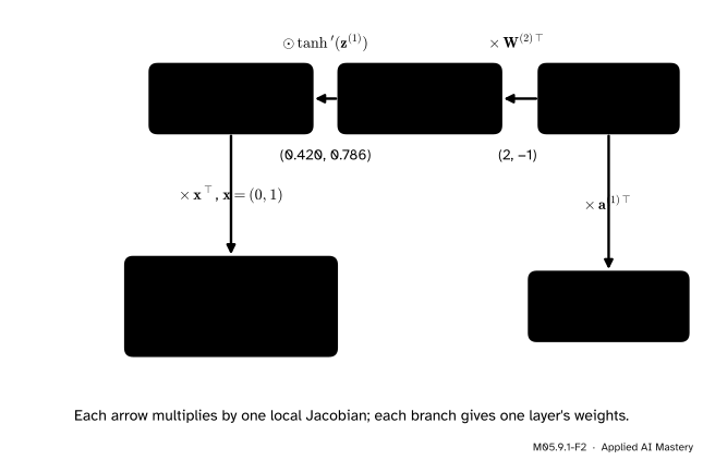
Step 4. Through the second layer.\(z^{(2)}\) uses each \(a^{(1)}_j\) once, with weight \(w^{(2)}_j\), so \({\partial \ell/\partial a^{(1)}_j} = {w^{(2)}_j\,\delta^{(2)}}\), and it uses each weight once, multiplied by \(a^{(1)}_j\), so \({\partial \ell/\partial w^{(2)}_j} = {\delta^{(2)} a^{(1)}_j}\).
Step 5. Through tanh. Each hidden unit has a single input, so its local Jacobian is diagonal: multiply entry by entry by \({\tanh'(z)} = {1 - \tanh^2 z} = {1 - a^2}\). This gives \({\vect{\delta}^{(1)}} = {\partial \ell/\partial \vect{z}^{(1)}}\).
Step 6. Into the first layer.\(z^{(1)}_j\) uses \(w^{(1)}_{jk}\) once, multiplied by \(x_k\), so \({\partial \ell/\partial w^{(1)}_{jk}} = {\delta^{(1)}_j x_k}\).
M05.9.1-F2
The backward pass as a chain read right to left. Each arrow multiplies by one local Jacobian: \(\mat{W}^{(2)\top}\), then the diagonal of \(\tanh'\). Each branch down to a layer’s weights multiplies by the value that entered that layer.
The formal statement
NoteBackpropagation for one example
For the network above, with the values of a forward pass recorded,
where \(\odot\) is the entrywise product and \(\vect{\delta}^{(l)}\) is the adjoint of \(\vect{z}^{(l)}\). These are the adjoint recurrence of M05.8.3 on the network’s graph.
Derivation. Every line is the recurrence \({\delta_{v}} = {\sum_{\text{children } u} \delta_u\, \partial u/\partial v}\), applied to one node at a time, from the loss backwards.
The output. The loss depends on \(z^{(2)}\) only through \(p\). Differentiating the log loss,
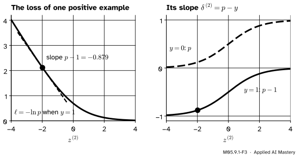
The sigmoid has \({\sigma'(z)} = {\sigma(z)(1 - \sigma(z))}\) (M04.3.3), so \({\partial p/\partial z^{(2)}} = {p(1 - p)}\). The product of the two is \({\delta^{(2)} = p - y}\): the factor \(p(1 - p)\) cancels.
M05.9.1-F3
The output adjoint is the predicted probability minus the label. It is large when the prediction is confidently wrong and near zero when it is right, which is what learning needs.
The second layer.\(z^{(2)} = {w^{(2)}_1 a^{(1)}_1} + {w^{(2)}_2 a^{(1)}_2} + b^{(2)}\) has local derivatives \({\partial z^{(2)}/\partial a^{(1)}_j} = {w^{(2)}_j}\), \({\partial z^{(2)}/\partial w^{(2)}_j} = {a^{(1)}_j}\) and \({\partial z^{(2)}/\partial b^{(2)}} = {1}\). \(z^{(2)}\) is the only child of each of these, so each adjoint is \({\delta^{(2)}}\) times one local derivative. In vectors: \({\partial\ell/\partial\vect{a}^{(1)}} = {\mat{W}^{(2)\top}\delta^{(2)}}\) and \({\nabla_{\mat{W}^{(2)}}\ell} = {\delta^{(2)}\vect{a}^{(1)\top}}\).
The hidden units.\({a^{(1)}_j = \tanh z^{(1)}_j}\) is the only child of \(z^{(1)}_j\), with local derivative \({1 - \tanh^2 z^{(1)}_j} = {1 - (a^{(1)}_j)^2}\), so \({\delta^{(1)}_j} = {(\partial\ell/\partial a^{(1)}_j)(1 - (a^{(1)}_j)^2)}\). Written as a Jacobian, the tanh layer is the diagonal matrix \({\operatorname{diag}(1 - (a^{(1)}_j)^2)}\), and multiplying a vector by a diagonal matrix is the entrywise product.
The first layer.\({z^{(1)}_j} = {\sum_k w^{(1)}_{jk} x_k} + {b^{(1)}_j}\), so \({\partial z^{(1)}_j/\partial w^{(1)}_{jk}} = {x_k}\) and the weight’s only child is \(z^{(1)}_j\): \({\partial\ell/\partial w^{(1)}_{jk}} = {\delta^{(1)}_j x_k}\), the entry \((j, k)\) of \({\vect{\delta}^{(1)}\vect{x}\T}\). The bias has local derivative 1.
Read as a whole, the backward pass multiplies a row vector by one local Jacobian after another,
from the left, the cheap order of M05.8.4. This is the picture of Mathematics for Machine Learning, section 5.6.1, where the gradient of each layer’s parameters reuses the products already formed for the layers after it.
Worked example
Every number for \({\vect{x} = (0, 1)}\), \({y = 1}\), to three decimals.
M05.9.1-F4
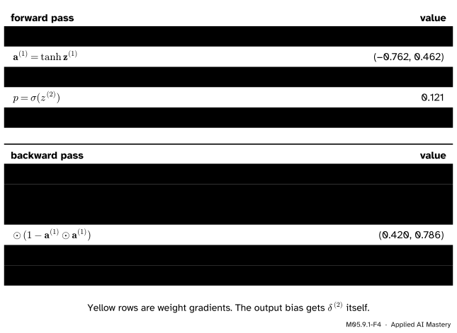
The worked trace. Read the forward block downwards, then the backward block downwards: each line uses only the line above it and values recorded on the way forward.
Forward.\({z^{(1)}_1} = {1 \cdot 0} + {(-1) \cdot 1} = {-1}\) and \({z^{(1)}_2} = {0.5 \cdot 0} + {0.5 \cdot 1} = {0.5}\). Then \({a^{(1)}_1} = {\tanh(-1)} \approx {-0.762}\) and \({a^{(1)}_2} = {\tanh 0.5} \approx {0.462}\). The score is \({z^{(2)}} = {2(-0.762)} + {(-1)(0.462)} \approx {-1.985}\), so \({p} = {1/(1 + e^{1.985})} \approx {0.121}\) and \({\ell = -\ln 0.121 \approx 2.114}\).
Backward.
\({\delta^{(2)}} = {p - 1} \approx {-0.879}\), which is also the gradient of \(b^{(2)}\).
The tanh slopes are \({1 - 0.762^2 \approx 0.420}\) and \({1 - 0.462^2 \approx 0.786}\), so \({\vect{\delta}^{(1)}} \approx {(-0.739,\ 0.691)}\), also the gradient of \(\vect{b}^{(1)}\).
\({\nabla_{\mat{W}^{(1)}}\ell} = {\vect{\delta}^{(1)}\,(0,\ 1)}\) has first column 0 and second column \({(-0.739,\ 0.691)}\).
Each value was computed from unrounded numbers; working with the rounded ones can move the last digit.
What the numbers say: \(w^{(1)}_{12}\) has gradient \(-0.739\), so the loss falls as it rises, and a step of gradient descent raises it; \(w^{(2)}_1\) has gradient 0.670, so the step lowers it. Every weight moves against its own gradient (the update rule of ML01.5.2), and M05.9.2 runs that rule.
Code
From scratch first, with the Var class of M05.8.3: the network is just a program, so building the loss from Var objects records the tape, and one call to backward fills in all nine adjoints.
import mathimport numpy as npclass Var:"""A scalar that remembers its parents and the local derivative to each one (M05.8.3)."""def__init__(self, value, parents=()):self.value, self.parents, self.adjoint = value, parents, 0.0@staticmethoddef lift(x):return x ifisinstance(x, Var) else Var(x)def__add__(self, other): o = Var.lift(other)return Var(self.value + o.value, ((self, 1.0), (o, 1.0)))__radd__=__add__def__mul__(self, other): o = Var.lift(other)return Var(self.value * o.value, ((self, o.value), (o, self.value)))__rmul__=__mul__def backward(self): order, seen, stack = [], set(), [(self, False)]while stack: # topological order v, finished = stack.pop()if finished: order.append(v)elifid(v) notin seen: seen.add(id(v)) stack.append((v, True)) stack += [(p, False) for p, _ in v.parents ifid(p) notin seen]for v in order: v.adjoint =0.0self.adjoint =1.0for v inreversed(order):for parent, local in v.parents: parent.adjoint += v.adjoint * local # add, never overwritedef tanh(v): th = math.tanh(v.value)return Var(th, ((v, 1- th * th),))def sigmoid(v): s =1/ (1+ math.exp(-v.value))return Var(s, ((v, s * (1- s)),))def log(v):return Var(math.log(v.value), ((v, 1/ v.value),))def log_loss(x, y, W1, b1, W2, b2):"""The running network on one example, built from Var objects.""" a1 = [tanh(W1[j][0] * x[0] + W1[j][1] * x[1] + b1[j]) for j inrange(2)] p = sigmoid(W2[0] * a1[0] + W2[1] * a1[1] + b2)return (-1.0) * log(p) if y ==1else (-1.0) * log(1.0+ (-1.0) * p), pW1 = [[Var(1.0), Var(-1.0)], [Var(0.5), Var(0.5)]]b1 = [Var(0.0), Var(0.0)]W2 = [Var(2.0), Var(-1.0)]b2 = Var(0.0)loss, p = log_loss((0.0, 1.0), 1, W1, b1, W2, b2)loss.backward()grad_W1 = np.array([[w.adjoint for w in row] for row in W1])grad_W2 = np.array([w.adjoint for w in W2])print(f"p = {p.value:.3f}, loss = {loss.value:.3f}")print("grad W1 =", np.round(grad_W1, 3).tolist(), " grad b1 =", [round(b.adjoint, 3) for b in b1])print("grad W2 =", np.round(grad_W2, 3).tolist(), " grad b2 =", round(b2.adjoint, 3))
p = 0.121, loss = 2.114
grad W1 = [[0.0, -0.739], [0.0, 0.691]]  grad b1 = [-0.739, 0.691]
grad W2 = [0.67, -0.406]  grad b2 = -0.879
The same derivatives with the chain rule written out by hand, in NumPy: the six lines of the formal statement.
delta2 = -0.879  delta1 = [-0.739  0.691]
agrees with the Var class: True
Finally the independent check: nudge one weight up and down by \({h = 10^{-5}}\) and difference the loss (M05.2.4). Here for \(w^{(1)}_{12}\) and \(w^{(1)}_{22}\) and the two weights of the second layer.
w1_12 central difference -0.738521  backprop -0.738521
w1_22 central difference 0.691481  backprop 0.691481
w2_1 central difference 0.669628  backprop 0.669628
w2_2 central difference -0.406314  backprop -0.406314
The two agree to about ten decimal places, the accuracy a central difference can give. In a library the same backward pass is one call, loss.backward() in PyTorch (DL01.7); DL01.5 does it by hand for bigger networks.
Explore
The module’s interactive, the Backprop stepper, is in M05.9.2. Choose the example \({(0, 1)}\) there and step through the forward and backward passes: every number of the worked example appears on the graph, node by node, and the table of weight gradients fills in beside a central-difference check. Then pick \({(0, 0)}\) and notice that only the biases get a gradient.
Pitfalls
M05.9.1-F5
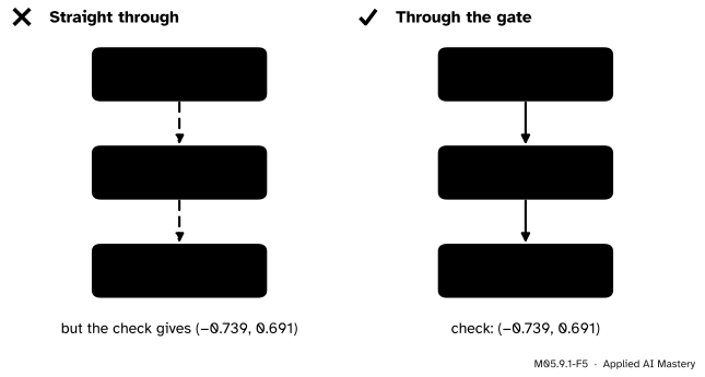
Wrong beside right. The tanh layer is a node of the graph, with its own local derivative. Skipping it more than doubles the first entry of \(\vect{\delta}^{(1)}\) here and gets the gradient of the first layer wrong.
“The hidden layer just passes the adjoint through.”
Every node on the path multiplies by its own local derivative, and an activation is a node. Without \({1 - a^2}\) the first-layer adjoint is \({(-1.758,\ 0.879)}\) instead of \({(-0.739,\ 0.691)}\). A gradient check catches it at once (M05.9.3).
“The output adjoint is always p minus y.”
It is \({p - y}\) because the log loss and the sigmoid fit together and \(p(1 - p)\) cancels. With the squared error \({(p - y)^2}\) the adjoint is \({2(p - y)\,p(1 - p)}\), which for our example is only about \(-0.187\): the confidently wrong output learns slowly (Exercise 2).
“A zero gradient means that weight is finished.”
\(w^{(1)}_{11}\) and \(w^{(1)}_{21}\) get 0 here only because \({x_1 = 0}\) in this example, so they have no effect on its loss. Over the whole batch they do get a gradient, from the examples with \({x_1 = 1}\). One example tells you about one example.
“Update the second layer, then backpropagate with its new weights.”
The backward pass uses the weights and values of the forward pass that recorded the tape. Change \(\mat{W}^{(2)}\) first and \({\mat{W}^{(2)\top}\delta^{(2)}}\) is the slope of a different network. Compute every gradient, then update every weight.
Check yourself
Recall
1. What is backpropagation, in the language of M05.8?
Show answer
Reverse-mode automatic differentiation applied to the loss of a network as a function of its weights: a recorded forward pass, then adjoints swept back from the loss.
2. For a sigmoid output with the log loss, what is the adjoint of the output score \(z^{(2)}\)?
Show answer
\({\delta^{(2)} = p - y}\), the predicted probability minus the label.
3. How does an adjoint pass through a tanh layer?
Show answer
Multiply entry by entry by \({1 - a^2}\), the slope of tanh at each unit’s input, written with the recorded output \(a\).
4. What is the gradient of a weight matrix of a dense layer for one example?
Show answer
The outer product \({\vect{\delta}\,\vect{a}_{\text{in}}\T}\) of the layer’s output adjoint and the value that entered the layer: \({\vect{\delta}^{(1)}\vect{x}\T}\) for the first layer.
5. Why do the weights from \(x_1\) get a zero gradient for the example \({(0, 1)}\)?
Show answer
Their gradient is \({\delta^{(1)}_j x_1}\) and \({x_1 = 0}\): changing them does not change this example’s loss.
Exercises
1.★ Run the forward and backward pass by hand for the example \({(1, 1)}\) with label 0, and give all nine gradients.
Show solution
Forward: \({\vect{z}^{(1)}} = {(1 - 1,\ 0.5 + 0.5)} = {(0, 1)}\), \({\vect{a}^{(1)} \approx (0, 0.762)}\), \({z^{(2)} \approx -0.762}\), \({p \approx 0.318}\) and \({\ell = -\ln(1 - p) \approx 0.383}\). Backward: \({\delta^{(2)} = p - 0 \approx 0.318}\), which is also the gradient of \(b^{(2)}\), and \({\nabla_{\mat{W}^{(2)}}\ell} \approx {0.318 \times (0, 0.762)} = {(0, 0.242)}\). Then \({\mat{W}^{(2)\top}\delta^{(2)}} \approx {(0.637, -0.318)}\), and the tanh slopes are 1 and \({1 - 0.762^2 \approx 0.420}\), so \({\vect{\delta}^{(1)}} \approx {(0.637, -0.134)}\), the gradient of \(\vect{b}^{(1)}\). With \({\vect{x} = (1, 1)}\) both columns of \({\vect{\delta}^{(1)}\vect{x}\T}\) equal \(\vect{\delta}^{(1)}\): rows \({(0.637,\ 0.637)}\) and \({(-0.134,\ -0.134)}\).
2.★★ Replace the log loss by the squared error \({\ell = (p - y)^2}\). Derive the output adjoint, evaluate it for the example \({(0, 1)}\) and compare it with \({p - y}\).
Show solution
\({\partial\ell/\partial p = 2(p - y)}\) and \({\partial p/\partial z^{(2)}} = {p(1 - p)}\), so \({\delta^{(2)} = 2(p - y)\,p(1 - p)}\). With \({p \approx 0.121}\): \({2 \times (-0.879) \times 0.121 \times 0.879} \approx {-0.187}\), against \(-0.879\) for the log loss. The factor \({p(1 - p)}\) is small whenever the sigmoid is confident, so when it is confidently wrong the squared error gives it only a small push. The log loss cancels that factor.
3.★★★ A network has layers \({\vect{z}^{(l)}} = {\mat{W}^{(l)}\vect{a}^{(l-1)}} + {\vect{b}^{(l)}}\) and \({\vect{a}^{(l)} = g(\vect{z}^{(l)})}\) entry by entry, with \({\vect{a}^{(0)} = \vect{x}}\). From the adjoint recurrence of M05.8.3, derive \({\vect{\delta}^{(l)}} = {(\mat{W}^{(l+1)\top}\vect{\delta}^{(l+1)}) \odot g'(\vect{z}^{(l)})}\) and \({\nabla_{\mat{W}^{(l)}}\ell} = {\vect{\delta}^{(l)}\vect{a}^{(l-1)\top}}\).
Show solution
The children of \(a^{(l)}_j\) are the entries \(z^{(l+1)}_i\), with local derivative \({\partial z^{(l+1)}_i/\partial a^{(l)}_j} = {w^{(l+1)}_{ij}}\). The recurrence gives \({\partial\ell/\partial a^{(l)}_j} = {\sum_i \delta^{(l+1)}_i w^{(l+1)}_{ij}}\), which is entry \(j\) of \({\mat{W}^{(l+1)\top}\vect{\delta}^{(l+1)}}\). The only child of \(z^{(l)}_j\) is \(a^{(l)}_j\), with local derivative \({g'(z^{(l)}_j)}\), so \({\delta^{(l)}_j}\) is that entry times \({g'(z^{(l)}_j)}\): the entrywise product. Finally the only child of \(w^{(l)}_{jk}\) is \(z^{(l)}_j\), with local derivative \(a^{(l-1)}_k\), so \({\partial\ell/\partial w^{(l)}_{jk}} = {\delta^{(l)}_j a^{(l-1)}_k}\), the entry \((j, k)\) of \({\vect{\delta}^{(l)}\vect{a}^{(l-1)\top}}\).
Summary card
Backpropagation is reverse mode on the graph of a network’s loss.
M05.9.1-F1
Forward values, then adjoints.
Output: \({\delta^{(2)} = p - y}\) for a sigmoid with the log loss.
Through a dense layer: multiply by \({\mat{W}\T}\).
Sources. Each was opened and checked against this lesson on 15 November 2026.
A. G. Baydin, B. A. Pearlmutter, A. A. Radul and J. M. Siskind, Automatic Differentiation in Machine Learning: a Survey, JMLR 18(153), 2018. Figure 1 shows backpropagation as a forward pass followed by an error adjoint propagated backward to the weights; section 3.2 says that reverse mode corresponds to a generalised backpropagation, with the output taken as the error \(E\); section 4.2 states that backpropagation is only a special case of reverse mode applied to a network’s error. Their adjoint \(\bar v\) is our \(\delta_v\).
M. P. Deisenroth, A. A. Faisal and C. S. Ong, Mathematics for Machine Learning, section 5.6.1: a deep network as a composition of layers \({\vect{f}_i} = {\sigma(\mat{A}_{i-1}\vect{f}_{i-1} + \vect{b}_{i-1})}\) (equation 5.113), the chain-rule products for each layer’s parameters (equations 5.115 to 5.118) and the remark that most of the computation is reused from the layers after; section 5.6.2: backpropagation is a special case of automatic differentiation, and reverse mode is the order of equation (5.120).