The determinant of the Jacobian is the factor by which a smooth map scales small areas near a point. Measure it for polar coordinates and the running warp, and see why a non-zero determinant lets a map be undone near a point, with the inverse matrix as the inverse’s Jacobian.
M05.4.4L2 Intermediate25 minIn review (what this means)
The maths and code on this page are checked by automated tests on every change, but an independent reader has not signed it off yet. Spot a mistake or a confusing step? Tell us.
Explain why |det J| is the limit of the area ratio of a small square and its image, and what the sign of det J means.
Derive det J = r for polar coordinates and check it against the exact area of a small polar cell.
State the inverse function theorem and derive, from the chain rule, that the Jacobian of a local inverse is the inverse matrix.
Measure area ratios of small squares numerically and find a local inverse with scipy.optimize.root.
The question
A normalising flow turns simple random points into realistic data by pushing them through a smooth map. To keep the probabilities right it must know, at every point, how much the map stretches or squeezes a tiny region. How do you read that off the map, and when can such a map be run backwards?
From the last lesson
1. What is the Jacobian of \({f \circ g}\) at \(\vect{a}\)?
Show answer
\({\mat{J}_f(g(\vect{a}))\,\mat{J}_g(\vect{a})}\): the outer Jacobian, evaluated at \({g(\vect{a})}\), on the left.
2. What is the Jacobian of tanh applied to each entry of a vector \(\vect{z}\)?
Show answer
\({\mathrm{diag}(1 - \tanh^2 z_i)}\), a diagonal matrix, because each output depends only on its own input.
Intuition
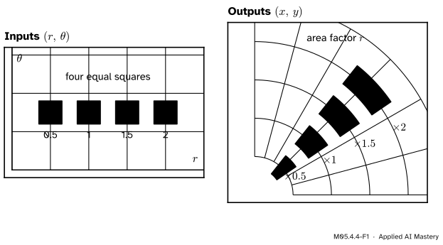
Lay four equal small squares in a row in the \({(r, \theta)}\) plane and send them through the polar map. They come out as curved cells of an annulus, and the further out they sit, the bigger they are.
M05.4.4-F1
Four equal squares in \({(r, \theta)}\) and their images. A square centred at radius \(r\) comes out with \(r\) times its area: the polar map’s Jacobian determinant.
Lesson M05.4.1 showed why: the polar Jacobian has a unit column pointing outwards and a column of length \(r\) pointing round the circle. A small square becomes, nearly, a rectangle \(r\) times as wide. The number that measures this stretch at each point is the determinant of the Jacobian.
Build it up
Step 1. A small square becomes a near-parallelogram. Take the square with sides \(s\) along the two axes and a corner at \(\vect{a}\). Its sides are \({s\vect{e}_1}\) and \({s\vect{e}_2}\); by M05.4.1 their images are about \({s\mat{J}\vect{e}_1}\) and \({s\mat{J}\vect{e}_2}\), the two columns of \(\mat{J}\) times \(s\).
Step 2. The parallelogram’s area. The area of the parallelogram spanned by two columns is the absolute value of the determinant of the matrix they form (M02.8). Scaling both columns by \(s\) scales the determinant by \(s^2\), so the area is \({s^2\,\abs{\det\mat{J}}}\).
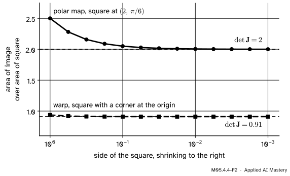
Step 3. Divide by the square’s area. The square has area \(s^2\), so the ratio of areas is about \({\abs{\det\mat{J}(\vect{a})}}\), and the approximation improves as \(s\) shrinks.
M05.4.4-F2
The measured area ratio of a shrinking square, for the polar map at \({(2, \pi/6)}\) and the running warp at the origin. Both settle on the Jacobian determinant.
Step 4. Polar cells, exactly. The image of the square \({[r, r + s] \times [\theta, \theta + s]}\) is the part of a sector of radius \({r + s}\) and angle \(s\) outside the sector of radius \(r\). A sector of radius \(R\) and angle \(s\) is the fraction \({s/(2\pi)}\) of a disc of area \({\pi R^2}\), so its area is \({sR^2/2}\), and
The ratio to the square’s area \(s^2\) is \({r + s/2}\), which tends to \(r\). At \({r = 2}\) it is 2.05 for \({s = 0.1}\) and 2.005 for \({s = 0.01}\).
The formal statement
NoteThe Jacobian determinant as an area factor
Let \(f\) map the plane to the plane with continuous partial derivatives near \(\vect{a}\). For squares \(S\) with a corner at \(\vect{a}\),
\[
\frac{\text{area of } f(S)}{\text{area of } S} \to \abs{\det\mat{J}_f(\vect{a})}
\]
as the side of \(S\) shrinks to 0. If \({\det\mat{J}_f(\vect{a}) > 0}\) the map keeps orientation near \(\vect{a}\); if it is negative it turns small shapes over, as a mirror does. The same holds in \(\R^n\) with volumes.
We state this without a full proof. The idea is Steps 1 to 3: the image’s boundary stays within a distance of the parallelogram’s boundary that is small compared with \(s\), so the two areas differ by a small fraction of \(s^2\). Lesson M05.6.4 uses exactly this factor to change variables in an integral.
The polar determinant. From the Jacobian of M05.4.1,
Let \(f\) map \(\R^n\) to \(\R^n\) with continuous partial derivatives near \(\vect{a}\), and suppose \({\det\mat{J}_f(\vect{a}) \neq 0}\). Then there are open sets \(U\) around \(\vect{a}\) and \(V\) around \({f(\vect{a})}\) such that \(f\) maps \(U\) one-to-one onto \(V\), the inverse \(g\) from \(V\) back to \(U\) has continuous partial derivatives, and
The existence of \(g\) is the deep part, and we take it from the theorem. The formula for its Jacobian then follows from the chain rule. For every \(\vect{x}\) in \(U\), \({g(f(\vect{x})) = \vect{x}}\). The identity map has Jacobian \(\mat{I}\), and by M05.4.3 the left side has Jacobian \({\mat{J}_g(f(\vect{a}))\,\mat{J}_f(\vect{a})}\). So their product is \(\mat{I}\), and a square matrix whose product with another is \(\mat{I}\) is that matrix’s inverse (M02.7).
M05.4.4-F3
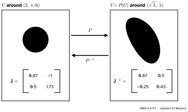
Near \({(2, \pi/6)}\) the polar map carries a small disc one-to-one onto an oval, and a local inverse carries it back, with the inverse matrix as its Jacobian.
For the polar map the local inverse is \({r = \sqrt{x^2 + y^2}}\) with \(\theta\) the angle of \({(x, y)}\). Its partial derivatives at \({(\sqrt3, 1)}\), where \({r = 2}\), are \({x/r \approx 0.866}\), \({y/r = 0.5}\), \({-y/r^2 = -0.25}\) and \({x/r^2 \approx 0.433}\): exactly the entries of \({\mat{J}_P(2, \pi/6)^{-1}}\). At \({r = 0}\) the determinant is 0 and the theorem says nothing; indeed every point \({(0, \theta)}\) goes to the origin, so no neighbourhood of \({(0, \theta)}\) is mapped one-to-one.
Frontier note: why normalising flows need log |det J|
A normalising flow writes data as \({\vect{x} = T(\vect{u})}\), with \(\vect{u}\) drawn from a simple density \({p_u}\) and \(T\) invertible and differentiable both ways. Probability is conserved: a small region keeps its probability while its area is multiplied by \({\abs{\det\mat{J}_T}}\), so the density is divided by that factor, \({p_x(\vect{x}) = p_u(\vect{u})\,\abs{\det\mat{J}_T(\vect{u})}^{-1}}\) (Papamakarios et al., Equation 2). In logs, \({\log p_x = \log p_u - \log\abs{\det\mat{J}_T}}\). A flow is a composition of many layers, so by the chain rule its log-determinant is a sum over layers (their Equation 28). Designs such as autoregressive and coupling layers make each Jacobian triangular, so its determinant is the product of the diagonal entries and costs only \(D\) operations in dimension \(D\) (their Equation 32). Change of variables for densities is M05.6.4 and M07.1; flows are DL06.7.
Worked example
The running warp. From \({\mat{J}_W = \begin{bmatrix} 1 & 0.3\cos y \\ 0.3\cos x & 1 \end{bmatrix}}\),
\[
\det\mat{J}_W = 1 - 0.09\cos x\cos y .
\]
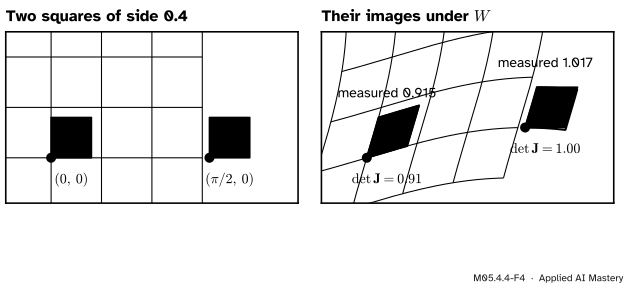
At \({(0, 0)}\) it is \({1 - 0.09 = 0.91}\): near the origin the warp shrinks areas by 9%. At \({(\pi/2, 0)}\) it is \({1 - 0 = 1}\): the shear there keeps areas. Since the product of the two cosines lies between \(-1\) and 1, the determinant always lies between 0.91 and 1.09. It is never 0, so the inverse function theorem gives a local inverse near every point.
M05.4.4-F4
The worked example as a trace. Squares of side 0.4 at the two points, and their images: the measured area ratios, 0.915 and 1.017, are already close to the determinants 0.91 and 1.
Measured. The exact image of a square of side 0.4 with a corner at \({(0, 0)}\) has 0.915 times its area; with side 0.01 the ratio is 0.91000. At \({(\pi/2, 0)}\) the ratios are 1.017 and 1.00045.
A local inverse. Near \({W(\pi/2, 0) = (\pi/2, 0.3)}\), which point is sent to \({(\pi/2 + 0.05,\; 0.28)}\), a step of \({\vect{\delta} = (0.05, -0.02)}\)? The inverse Jacobian answers to first order. Here
so the input moves by about \({\mat{J}_W^{-1}\vect{\delta}} = {(0.05 + 0.006,\; -0.02)} = {(0.056, -0.02)}\). Solving \({W(\vect{x}) = (\pi/2 + 0.05,\; 0.28)}\) exactly, as the code does, gives a move of about \({(0.0559, -0.0195)}\).
Code
From scratch: the exact image of a square is traced along its boundary and its area found with the shoelace formula, \({\tfrac12\sum (x_k y_{k+1} - x_{k+1}y_k)}\).
import numpy as npfrom scipy.optimize import rootdef warp(v): x, y = vreturn np.array([x +0.3* np.sin(y), y +0.3* np.sin(x)])def polar(v): r, th = vreturn np.array([r * np.cos(th), r * np.sin(th)])def square_boundary(corner, s, n=400): t = np.linspace(0, s, n, endpoint=False) x0, y0 = corner xs = np.concatenate([x0 + t, np.full(n, x0 + s), x0 + s - t, np.full(n, x0)]) ys = np.concatenate([np.full(n, y0), y0 + t, np.full(n, y0 + s), y0 + s - t])return np.array([xs, ys])def area_ratio(f, corner, s): x, y = f(square_boundary(corner, s)) area =0.5* np.sum(x * np.roll(y, -1) - np.roll(x, -1) * y)return area / s **2det_warp =lambda x, y: 1-0.09* np.cos(x) * np.cos(y)for corner in [(0.0, 0.0), (np.pi /2, 0.0)]: ratios = [round(area_ratio(warp, corner, s), 5) for s in (0.4, 0.1, 0.01)]print("warp at", np.round(corner, 3), "ratios", ratios, " det J", round(det_warp(*corner), 5))print("polar at (2, pi/6):", [round(area_ratio(polar, (2, np.pi /6), s), 5) for s in (0.1, 0.01)])
warp at [0. 0.] ratios [np.float64(0.9147), np.float64(0.9103), np.float64(0.91)]  det J 0.91
warp at [1.571 0.   ] ratios [np.float64(1.01729), np.float64(1.00449), np.float64(1.00045)]  det J 1.0
polar at (2, pi/6): [np.float64(2.05), np.float64(2.005)]
Now a local inverse. scipy.optimize.root solves \({W(\vect{x}) = \vect{y}}\) for \(\vect{x}\), starting from a guess; we start at \({(\pi/2, 0)}\). Differencing the solver’s answer in each coordinate of \(\vect{y}\) gives the Jacobian of the inverse, to compare with the inverse matrix.
a = np.array([np.pi /2, 0.0])J = np.array([[1.0, 0.3* np.cos(a[1])], [0.3* np.cos(a[0]), 1.0]])delta = np.array([0.05, -0.02])def inverse(y): sol = root(lambda v: warp(v) - y, a, tol=1e-13)assert sol.successreturn sol.xmove = inverse(warp(a) + delta) - aprint("exact move", move.round(4), " first-order", np.linalg.solve(J, delta).round(4))h =1e-5J_inv = np.column_stack([(inverse(warp(a) + h * e) - inverse(warp(a) - h * e)) / (2* h) for e in np.eye(2)])print("Jacobian of the inverse:\n", J_inv.round(6), "\ninverse of J:\n", np.linalg.inv(J).round(6))
exact move [ 0.0559 -0.0195]  first-order [ 0.056 -0.02 ]
Jacobian of the inverse:
 [[ 1.  -0.3]
 [ 0.   1. ]]
inverse of J:
 [[ 1.  -0.3]
 [-0.   1. ]]
Explore
This module’s interactive, the grid warp, lives in lesson M05.4.1. Choose the polar map and drag the point outwards: the measured area ratio follows \(r\). Then press Shrink the square and watch the ratio settle on \({\det\mat{J}}\), from \({r + s/2}\) down to \(r\).
Pitfalls
M05.4.4-F5
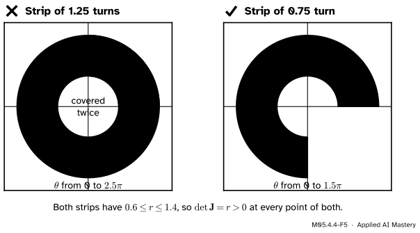
Wrong beside right. The polar map has \({\det\mat{J} = r > 0}\) on both strips, but the longer strip wraps round and lands on the same points twice.
“The determinant is never zero, so the map is one-to-one everywhere.”
The inverse function theorem is local. The polar map on the strip \({0.6 \le r \le 1.4}\), \({0 \le \theta \le 2.5\pi}\) has determinant \({r > 0}\) at every point, yet \({(1, \pi/4)}\) and \({(1, \pi/4 + 2\pi)}\) land on the same point. Near any one point it can be undone; over the whole strip it cannot.
“Where the determinant is zero, there is no inverse at all.”
A zero determinant only removes the guarantee. The map \({x \mapsto x^3}\) has derivative 0 at 0, yet it is one-to-one, with inverse the cube root. What fails is the inverse’s derivative: the cube root is not differentiable at 0. The polar map at \({r = 0}\), by contrast, really cannot be undone.
“The area factor is \({\det\mat{J}}\), so it can be negative.”
Area is never negative. The factor is \({\abs{\det\mat{J}}}\); the sign tells you about orientation. The swap \({(x, y) \mapsto (y, x)}\) has determinant \(-1\): it keeps every area and turns every shape over. Forgetting the absolute value gives negative probabilities in a change of variables.
Check yourself
Recall
1. What does \({\abs{\det\mat{J}_f(\vect{a})}}\) measure?
Show answer
The factor by which \(f\) scales small areas near \(\vect{a}\): the limit of the area of the image of a small square over the area of the square.
2. What is the Jacobian determinant of the polar map, and where is it zero?
Show answer
\(r\). It is zero at \({r = 0}\), where every angle is sent to the origin.
3. State the inverse function theorem in one sentence.
Show answer
If \(f\) has continuous partial derivatives near \(\vect{a}\) and \({\det\mat{J}_f(\vect{a}) \neq 0}\), then \(f\) can be undone near \(\vect{a}\) by a smooth local inverse, whose Jacobian at \({f(\vect{a})}\) is \({\mat{J}_f(\vect{a})^{-1}}\).
4. How does the chain rule give the Jacobian of the inverse?
Show answer
From \({g(f(\vect{x})) = \vect{x}}\): \({\mat{J}_g(f(\vect{a}))\,\mat{J}_f(\vect{a}) = \mat{I}}\), so \({\mat{J}_g(f(\vect{a})) = \mat{J}_f(\vect{a})^{-1}}\).
5. What does a negative Jacobian determinant mean?
Show answer
The map turns small shapes over near the point, as a mirror does; it still scales area by the absolute value.
Exercises
1.★ Find the Jacobian determinants of \({(u, v) \mapsto (2u, 3v)}\) and of \({(u, v) \mapsto (u + v^2, v)}\).
Show solution
The first has Jacobian \({\mathrm{diag}(2, 3)}\), determinant 6: every area is multiplied by 6. The second has Jacobian \({\begin{bmatrix} 1 & 2v \\ 0 & 1 \end{bmatrix}}\), determinant 1 at every point: it bends the grid but keeps every area, like a shear.
2.★★ Let \({f(x, y) = (x^2 - y^2,\; 2xy)}\), the squaring of complex numbers (M01.9). Find \({\det\mat{J}_f}\). Where does the inverse function theorem fail, and is \(f\) one-to-one away from that point?
so \({\det\mat{J}_f = 4x^2 + 4y^2}\), which is zero only at the origin. Everywhere else \(f\) has a local inverse. But it is not one-to-one: \({f(1, 0) = f(-1, 0) = (1, 0)}\), since \(z\) and \(-z\) have the same square. Again the theorem is only local.
3.★★★ Find the Jacobian of the local inverse of the running warp at \({W(0, 0) = (0, 0)}\). Then show that the warp is one-to-one on the whole plane. (Use \({\abs{\sin p - \sin q} \le \abs{p - q}}\).)
Show solution
\({\mat{J}_W(0, 0) = \begin{bmatrix} 1 & 0.3 \\ 0.3 & 1 \end{bmatrix}}\) with determinant 0.91, so the inverse’s Jacobian is
Each entry of the bracket is at most the matching entry of \({(p_2 - q_2,\; p_1 - q_1)}\) in size, a vector of length \({\norm{\vect{p} - \vect{q}}}\). So \({\norm{\vect{p} - \vect{q}} \le 0.3\,\norm{\vect{p} - \vect{q}}}\), which forces \({\vect{p} = \vect{q}}\).
Summary card
The Jacobian determinant is the local area factor; where it is not zero, the map can be undone nearby.
M05.4.4-F1
Area factor \(r\) for polar cells.
Area of \({f(S)}\) over area of \(S\) tends to \({\abs{\det\mat{J}_f(\vect{a})}}\); the sign is orientation.
Polar: \({\det\mat{J} = r}\). Warp: \({1 - 0.09\cos x\cos y}\), from 0.91 to 1.09.
\({\det\mat{J}_f(\vect{a}) \neq 0}\): a local inverse \(g\), with \({\mat{J}_g(f(\vect{a})) = \mat{J}_f(\vect{a})^{-1}}\).
Local, not global: the polar map wraps round.
Sources and next steps
Sources. Each was opened and checked against this lesson on 15 November 2026.
Gilbert Strang and Edwin Herman, Calculus Volume 3 (OpenStax), Section 5.7: the book’s “Jacobian” is the determinant of this matrix; Example 5.67 finds \({J(r, \theta) = r}\) for polar coordinates, and Theorem 5.14 asks for a one-to-one map with a non-zero Jacobian.
Marc Peter Deisenroth, A. Aldo Faisal and Cheng Soon Ong, Mathematics for Machine Learning, Section 5.3: the absolute value of the Jacobian determinant is the factor by which areas or volumes are scaled, exact for a linear map and a local approximation for a nonlinear one.
Rasul Shafikov, Real Analysis lecture notes, Section 2 (University of Western Ontario): Theorem 2.4, the inverse function theorem, and the example \({x^3}\), whose inverse exists but is not differentiable at 0.
George Papamakarios, Eric Nalisnick, Danilo Jimenez Rezende, Shakir Mohamed and Balaji Lakshminarayanan, Normalizing Flows for Probabilistic Modeling and Inference, JMLR 22 (2021), Section 2.1 (Equations 2 to 6: the density under a map, the determinant as a volume ratio, composition), Equation 28 and Section 3.1 (Equation 32, triangular Jacobians).
SciPy 1.18 reference, scipy.optimize.root: arguments fun and x0, default method hybr, and the result’s x and success.
Next. Lesson M05.5.1 differentiates the gradient itself: the Jacobian of the gradient is the Hessian. Lesson M05.6.4 uses the area factor to change variables in an integral.