A smooth one-to-one map sends each small cell to a near-parallelogram whose area is |det J| times the cell’s. So integrals change variables with the factor |det J|, polar coordinates included, and a density pushed through a map is divided by it: the idea behind normalising flows.
M05.6.4L2 Intermediate25 minIn review (what this means)
The maths and code on this page are checked by automated tests on every change, but an independent reader has not signed it off yet. Spot a mistake or a confusing step? Tell us.
Explain why a small cell of area du dv is sent to a near-parallelogram of area |det J| du dv, and state the change-of-variables theorem with its conditions.
Recover dA = r dr dtheta as the case det J = r, and evaluate integrals over a parallelogram and an ellipse by straightening them into a square and a disc.
Derive the density of Y = T(X) from the density of X, and compute it for a linear map of two independent standard normals.
Check a change of variables numerically with scipy.integrate.dblquad in both coordinates and a transformed density against a histogram of samples.
The question
A normalising flow is a generative model that turns simple random noise into realistic data by pushing it through a smooth invertible map. To train it by maximum likelihood, it must know the density of what comes out. If the noise has a known density, what is the density after the map? The same question in calculus: when we change the variables of an integral, what replaces the \(r\) of \({r\,dr\,d\theta}\)?
From the last lesson
1. What is the exact area of the polar cell between radii \(r\) and \({r + \Delta r}\) and angles \(\theta\) and \({\theta + \Delta\theta}\)?
2. What is the integral of \({e^{-(x^2 + y^2)/2}}\) over the plane?
Show answer
\({2\pi}\), so the bell curve has area \({\sqrt{2\pi}}\).
Intuition
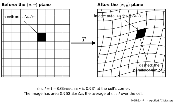
A map \(T\) from a \({(u, v)}\) plane to an \({(x, y)}\) plane bends the square grid into a curved one. Up close, though, a smooth map looks linear (M05.4.1), so each tiny cell lands on a tiny near-parallelogram, and a linear map scales areas by its determinant (M02.8).
M05.6.4-F1
The running warp \({(u, v)} \mapsto {(u + 0.3\sin v,\; v + 0.3\sin u)}\) of M05.4. A small cell (left) lands on a curved four-sided shape (right) that the parallelogram of the Jacobian matches closely. Its area is the cell’s area times \({\abs{\det J}}\).
So an integral over the curved region in \({(x, y)}\) can be done cell by cell in \({(u, v)}\), where the cells are squares, provided each cell’s value is multiplied by \({\abs{\det J}}\), the amount its area is stretched. For polar coordinates that factor was \(r\).
Build it up
Step 1. A map and two regions. Let \({T(u, v)} = {\big(x(u, v),\, y(u, v)\big)}\) be smooth and one-to-one on a region \(D\) of the \({(u, v)}\) plane, and let \({T(D)}\) be its image. Cut \(D\) into small cells; because \(T\) is one-to-one, their images tile \({T(D)}\) without overlapping.
Step 2. Where the corners go. Take the cell with corner \({(u, v)}\) and sides \({\Delta u}\), \({\Delta v}\). By the linear approximation of M05.4.1,
where \(\vect{j}_1\) and \(\vect{j}_2\) are the columns of the Jacobian \({\mat{J}_T(u, v)}\): the partial derivatives of \(T\) with respect to \(u\) and to \(v\).
Step 3. The image is nearly a parallelogram. So the image of the cell is close to the parallelogram spanned by \({\Delta u\,\vect{j}_1}\) and \({\Delta v\,\vect{j}_2}\). Its area is the absolute value of the determinant of those two columns (M02.8.1):
\[
\text{area} \approx \abs{\det \mat{J}_T(u, v)}\;\Delta u\,\Delta v .
\]
M05.6.4-F2
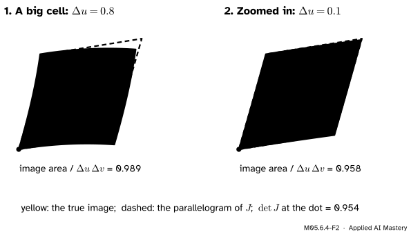
Zooming in. For a big cell the image bends away from the parallelogram; for a small one they almost coincide, and the area ratio, 0.958, approaches \({\det \mat{J} = 0.954}\) at the corner.
Step 4. Add up the cells. The integral of \(f\) over \({T(D)}\) is about the sum, over the cells, of \(f\) at the image of a corner times the image’s area:
\[
\sum f\big(T(u, v)\big)\,\abs{\det \mat{J}_T(u, v)}\,\Delta u\,\Delta v .
\]
That is a Riemann sum in \({(u, v)}\) over \(D\), and as the cells shrink it tends to an integral over \(D\).
The formal statement
NoteTheorem: change of variables in a double integral
Let \({T : D \to \R^2}\) be one-to-one, with continuous partial derivatives, and with \({\det \mat{J}_T \ne 0}\) inside \(D\). For \(f\) continuous on \({T(D)}\),
In short, \({dA = \abs{\det \mat{J}_T}\,du\,dv}\).
The build is the reason. A full proof must also show that the errors of Steps 2 and 3, small on each cell, stay small when added over many cells; continuity of the partial derivatives makes that work, and the source below states the theorem with exactly these conditions.
Polar coordinates again. For \({T(r, \theta) = (r\cos\theta,\; r\sin\theta)}\),
so \({\det \mat{J}_T = r\cos^2\theta + r\sin^2\theta = r}\). The theorem gives \({dA = r\,dr\,d\theta}\), the result of M05.6.3.
Linear maps. For \({T(\vect{u}) = \mat{A}\vect{u}}\) the Jacobian is \(\mat{A}\) everywhere, and with \({f = 1}\) the theorem says \({\text{area}(T(D))} = {\abs{\det \mat{A}}\,\text{area}(D)}\), the area factor of M02.8, now for any region. In one variable it is the substitution rule of M04.7.1: \({\int f(g(u))\,\abs{g'(u)}\,du}\), where the absolute value takes the place of turning the limits round.
Densities. Let a random point \({X = (X_1, X_2)}\) have density \(p_X\), and let \({Y = T(X)}\) for a one-to-one smooth \(T\) with a smooth inverse. For any region \(B\), \({Y}\) is in \(B\) exactly when \(X\) is in \({T^{-1}(B)}\), so
\[
\Prob(Y \in B) = \iint_{T^{-1}(B)} p_X\,dA .
\]
Change variables in this integral with the map \({T^{-1}}\), which carries \(B\) onto \({T^{-1}(B)}\):
By the inverse function theorem (M05.4.4), \({\mat{J}_{T^{-1}}(\vect{y})}\) is the inverse of \({\mat{J}_T(\vect{x})}\) at \({\vect{x} = T^{-1}(\vect{y})}\), and the determinant of an inverse is the reciprocal of the determinant. So equally \({p_Y(\vect{y})} = {p_X(\vect{x}) \,/\, \abs{\det \mat{J}_T(\vect{x})}}\): where the map spreads area out, the density thins in proportion. For a linear map this is the formula of M02.8.4, now proved for any smooth one-to-one map.
A linear map of two standard normals. Let \(X_1\) and \(X_2\) be independent standard normals, so \({p_X(\vect{x}) = \tfrac{1}{2\pi} e^{-\norm{\vect{x}}^2/2}}\), a density by M05.6.3. Push them through the running matrix \(\mat{T}\) of M02, with rows \({(1, 1)}\) and \({(-1, 2)}\) and \({\det \mat{T} = 3}\):
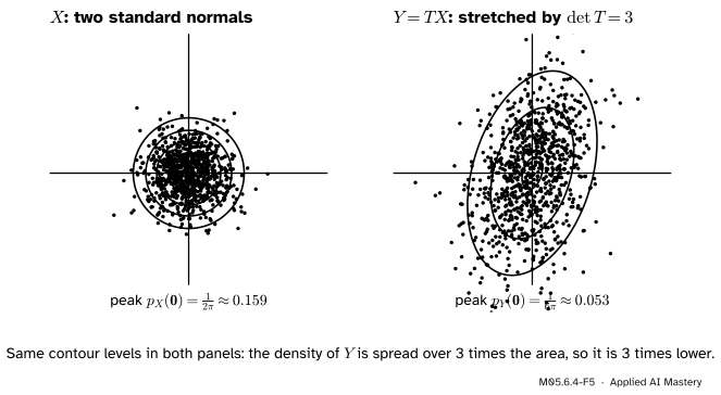
At the origin it is \({\tfrac{1}{6\pi} \approx 0.053}\), a third of \({p_X(\vect{0}) \approx 0.159}\). At \({\vect{y} = (1, 2)}\), \({\mat{T}^{-1}\vect{y} = (0, 1)}\) and \({p_Y = e^{-1/2}/(6\pi) \approx 0.032}\). Course M07 recognises this as the normal density with covariance \({\mat{T}\mat{T}\T}\) (M07.1, M07.3).
M05.6.4-F5
A density through a map. The cloud is stretched over three times the area, so its density, drawn with the same contour levels, is three times lower: the innermost level of the left panel is not reached at all on the right.
Worked example
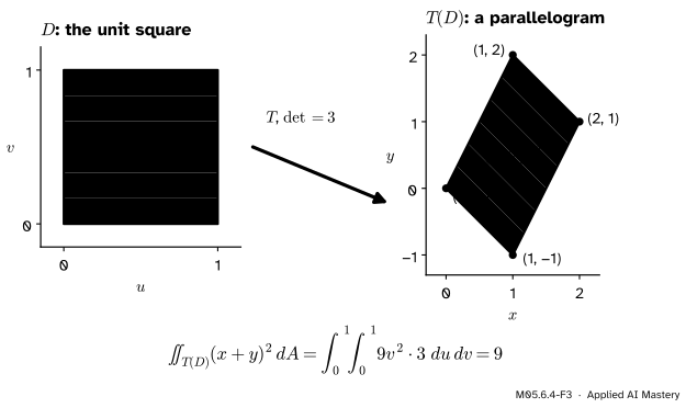
A parallelogram, straightened. Integrate \({(x + y)^2}\) over the parallelogram with corners \({(0, 0)}\), \({(1, -1)}\), \({(2, 1)}\) and \({(1, 2)}\). In Cartesian coordinates its edges change at \({x = 1}\), so it needs two pieces. But it is the image of the unit square under the running linear map, \({x = u + v}\) and \({y = -u + 2v}\): the corners \({(0,0)}\), \({(1,0)}\), \({(1,1)}\) and \({(0,1)}\) go to the four corners above. Then \({x + y = 3v}\), \({\abs{\det \mat{J}}} = {\abs{1 \cdot 2 - 1 \cdot (-1)}} = 3\), and
With \({f = 1}\) instead, the area of the parallelogram is \({3 \times 1 = 3}\).
M05.6.4-F3
The straightening. Each horizontal band of the square (left) lands on a slanted band of the parallelogram (right) along which \({x + y = 3v}\) is constant, so the integrand depends on \(v\) alone.
An ellipse, rounded. The region \({x^2/a^2 + y^2/b^2 \le 1}\) is the image of the unit disc under \({x = au}\), \({y = bv}\), whose Jacobian is \({\operatorname{diag}(a, b)}\) with determinant \({ab}\). So its area is \({ab \times \pi}\). The region where the running bowl is at most 2, \({x^2 + 2y^2 \le 2}\), is the ellipse with \({a = \sqrt2}\) and \({b = 1}\), of area \({\sqrt2\,\pi \approx 4.443}\).
Code
The parallelogram in both coordinates. Directly, the lower edge is the larger of \({y = -x}\) and \({y = 2x - 3}\) and the upper edge the smaller of \({y = 2x}\) and \({y = 3 - x}\).
The transformed density, from scratch, then checked two ways: against the normal density with covariance \({\mat{T}\mat{T}\T}\), and against samples. The fraction of samples of \(Y\) that land in a small square should match the integral of \(p_Y\) over it, up to sampling noise.
T = np.array([[1.0, 1.0], [-1.0, 2.0]])T_inv = np.linalg.inv(T)def p_X(x):return math.exp(-(x @ x) /2) / (2* math.pi)def p_Y(y):return p_X(T_inv @ y) *abs(np.linalg.det(T_inv)) # density through the mapS = T @ T.T # covariance of Y, [[2, 1], [1, 5]]gauss =lambda y: math.exp(-0.5* y @ np.linalg.solve(S, y)) / (2* math.pi * math.sqrt(np.linalg.det(S)))for y in [np.zeros(2), np.array([1.0, 2.0]), np.array([-1.5, 0.5])]:print(y, round(p_Y(y), 5), round(gauss(y), 5))rng = np.random.default_rng(0)Y = rng.standard_normal((400_000, 2)) @ T.T # samples of Y = T Xbox = (0.5, 1.5, 1.5, 2.5) # 0.5 < y1 < 1.5, 1.5 < y2 < 2.5inside = np.mean((Y[:, 0] >0.5) & (Y[:, 0] <1.5) & (Y[:, 1] >1.5) & (Y[:, 1] <2.5))exact = dblquad(lambda y2, y1: p_Y(np.array([y1, y2])), 0.5, 1.5, 1.5, 2.5)[0]noise = math.sqrt(exact * (1- exact) /len(Y))print("samples:", round(inside, 4), " integral of p_Y:", round(exact, 4), " noise about", round(noise, 4))
[0. 0.] 0.05305 0.05305
[1. 2.] 0.03218 0.03218
[-1.5  0.5] 0.02541 0.02541
samples: 0.0318  integral of p_Y: 0.0314  noise about 0.0003
The last check is statistical: with a different random generator the fraction would change in its third decimal place, but it stays within a few standard errors of the integral.
Explore
The region integrator in lesson M05.6.3 shows the special case of this lesson for polar coordinates. Pick the disc and polar cells: the read-out gives the areas of a yellow cell near the centre and one at the rim, and their ratio is the ratio of their radii, which is \({\det \mat{J} = r}\) at work.
Pitfalls
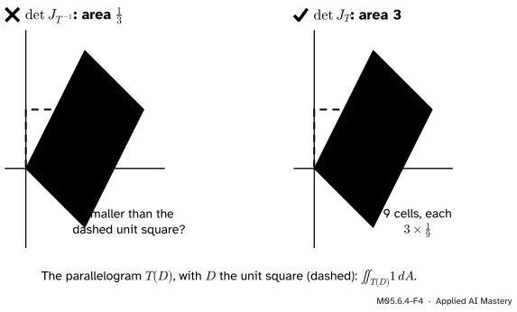
M05.6.4-F4
Wrong beside right. The parallelogram plainly covers more than the unit square, so its area cannot be \({\tfrac13}\). The factor comes from the map from the variables you integrate in, \({(u, v)}\), to the old ones, \({(x, y)}\).
“Use the Jacobian of the new variables in terms of the old ones.”
In \({\iint_{T(D)} f\,dA} = {\iint_D f(T)\,\abs{\det \mat{J}_T}\,du\,dv}\), the Jacobian is that of \(T\), which writes the old variables \(x\), \(y\) in terms of the new ones \(u\), \(v\). If you have the new variables as functions of the old, \({u = \tfrac{2x - y}{3}}\) and \({v = \tfrac{x + y}{3}}\) here, their Jacobian has determinant \({\tfrac13}\), and you need its reciprocal, 3.
“The factor is \(\det \mat{J}\).”
It is \({\abs{\det \mat{J}}}\). Areas are positive, but a map that flips orientation, such as \({(u, v) \mapsto (v, u)}\) with determinant \(-1\), has a negative determinant. Without the absolute value the area of the unit square under that swap would come out as \(-1\).
“Any map will do.”
The map must be one-to-one on \(D\), or some of \({T(D)}\) is counted twice. Polar coordinates with \({0 \le \theta \le 4\pi}\) sweep the disc twice and give \({2\pi a^2}\) for its area. In a density the same mistake gives a total probability of 2.
Frontier note: normalising flows: log-likelihoods through a map
A normalising flow writes data as \({\vect{x} = T(\vect{u})}\) with \(\vect{u}\) drawn from a simple base density. Equations (2) and (3) of Papamakarios and colleagues are the density formula above, in both of its forms. Taking logs, \({\log p_X(\vect{x})} = {\log p_U(\vect{u})} - {\log\abs{\det \mat{J}_T(\vect{u})}}\), and for a chain of maps the log-determinants add. Training maximises this, so flows use maps whose Jacobian determinant is cheap, for example with a triangular Jacobian, whose determinant is the product of its diagonal (DL06.7). Lesson M05.7.4 derives the gradient of \({\log\abs{\det}}\) that such training needs.
Check yourself
Recall
1. A small cell of area \({\Delta u\,\Delta v}\) is mapped by \(T\). About what area does its image have?
Show answer
\({\abs{\det \mat{J}_T(u, v)}\,\Delta u\,\Delta v}\): the area of the parallelogram spanned by the Jacobian’s columns times \({\Delta u}\) and \({\Delta v}\).
2. State the change-of-variables formula and its conditions.
Show answer
\({\iint_{T(D)} f\,dA} = {\iint_D f(T(u, v))\,\abs{\det \mat{J}_T}\,du\,dv}\), for \(T\) one-to-one with continuous partial derivatives and non-zero Jacobian determinant inside \(D\), and \(f\) continuous.
3. What is \({\det \mat{J}}\) for polar coordinates?
Show answer
\(r\), so \({dA = r\,dr\,d\theta}\).
4. What is the density of \({Y = T(X)}\)?
Show answer
\({p_Y(\vect{y})} = {p_X(T^{-1}(\vect{y}))\,\abs{\det \mat{J}_{T^{-1}}(\vect{y})}}\), which equals \({p_X(\vect{x})/\abs{\det \mat{J}_T(\vect{x})}}\) at \({\vect{x} = T^{-1}(\vect{y})}\).
5. Two standard normals are pushed through a linear map with determinant 3. What is the density of the result at the origin?
1.★ Find the area of the ellipse \({x^2/9 + y^2/4 \le 1}\).
Show solution
With \({x = 3u}\), \({y = 2v}\) the ellipse is the image of the unit disc and \({\det \mat{J} = 6}\), so its area is \({6\pi \approx 18.85}\).
2.★★ Let \(R\) be the square with corners \({(0, 0)}\), \({(1, 1)}\), \({(2, 0)}\) and \({(1, -1)}\). Compute \({\iint_R (x - y)^2\,dA}\) with \({u = x + y}\), \({v = x - y}\).
Show solution
The corners go to \({(u, v)} = {(0, 0)}\), \({(2, 0)}\), \({(2, 2)}\) and \({(0, 2)}\), so \(R\) becomes the square \({[0, 2]^2}\). Solving, \({x = \tfrac{u + v}{2}}\) and \({y = \tfrac{u - v}{2}}\), so
3.★★★ Let \(X\) be uniform on the unit square (density 1 there) and \({Y = \mat{A}X}\), where \(\mat{A}\) has rows \({(2, 0)}\) and \({(1, 1)}\). Find the density of \(Y\), check that it integrates to 1, and find \({\Prob(Y_1 < 1)}\).
Show solution
\({\det \mat{A} = 2}\), so \({p_Y(\vect{y}) = 1 \times \tfrac12 = \tfrac12}\) on the parallelogram \({\mat{A}([0, 1]^2)}\), with corners \({(0, 0)}\), \({(2, 1)}\), \({(2, 2)}\) and \({(0, 1)}\), and 0 elsewhere. The parallelogram has area \({2 \times 1 = 2}\), so the total is \({\tfrac12 \times 2 = 1}\). Finally \({Y_1 = 2X_1}\), so \({\Prob(Y_1 < 1)} = {\Prob(X_1 < \tfrac12)} = \tfrac12\); equally, the part of the parallelogram with \({y_1 < 1}\) has area 1, times the density \({\tfrac12}\).
Summary card
Change variables cell by cell: every cell’s area is stretched by \({\abs{\det \mat{J}}}\).
Sources. Each was opened and checked against this lesson on 15 November 2026.
Gilbert Strang and Edwin Herman, Calculus Volume 3, Section 5.7, Change of variables in multiple integrals, OpenStax. The Jacobian of a map of the plane, the image of a small rectangle with area about \({\abs{J}\,\Delta u\,\Delta v}\) found from the tangent vectors, and the change-of-variables theorem for a one-to-one map with continuous partial derivatives and non-zero Jacobian inside the region (Theorem 5.14); Example 5.70 integrates over a parallelogram by straightening it.
Marc Peter Deisenroth, A. Aldo Faisal and Cheng Soon Ong, Mathematics for Machine Learning, Cambridge University Press, 2020. Section 5.3 reads \({\abs{\det \mat{J}}}\) as the factor by which a map scales areas (its example has factor 3). Section 6.7, Theorem 6.16 (equation 6.144) gives the density of \({Y = U(X)}\) with the determinant of the Jacobian of the inverse, and Example 6.17 applies it to a linear map of a standard normal pair. The book writes Jacobians in the same layout as this course.
George Papamakarios, Eric Nalisnick, Danilo Jimenez Rezende, Shakir Mohamed and Balaji Lakshminarayanan, Normalizing Flows for Probabilistic Modeling and Inference, JMLR 22(57), 2021. Section 2.1, equations (2) and (3): the density of a flow’s output in terms of the base density and the Jacobian determinant of the map or of its inverse.
Next. M05.7 derives matrix gradients with differentials, ending with the derivative of \({\log\det}\) that flows need (M05.7.4). Course M07 transforms random variables in general (M07.1) and meets the multivariate normal, of which \({Y = \mat{T}X}\) above is one (M07.3).