Derive the Hessians of the mean squared error and of the logistic log loss, see why both are never negative, take the Newton step that lands on the least-squares answer in one move, and find the largest eigenvalue from Hessian-vector products: the curvature that caps the learning rate.
M05.5.4L2 Intermediate25 minIn review (what this means)
The maths and code on this page are checked by automated tests on every change, but an independent reader has not signed it off yet. Spot a mistake or a confusing step? Tell us.
Derive the Hessian (2/n) XᵀX of the mean squared error and the Hessian (1/n) XᵀSX of the mean log loss, and show that both are positive semidefinite.
Derive the Newton step -H⁻¹∇L as the minimiser of the Taylor model, and show that it solves least squares in one step from any start.
Compute a Hessian-vector product from two gradients and find the largest eigenvalue with the power method.
Explain why gradient descent on a quadratic is stable exactly when the learning rate is below 2/λ_max.
The question
Train the line \({\hat y = wx + b}\) on the four running points by gradient descent. How large can the learning rate be before the steps blow up instead of settling? And is there a step that lands on the best line \({(1.4, 0.5)}\) in one move, from anywhere? Both answers are written in the loss’s Hessian. The same number, its largest eigenvalue, is the sharpness that deep-learning practice watches during training.
From the last lesson
1. State the verdict for each sign pattern of the eigenvalues of \(\mat{H}\) at a critical point.
Show answer
All positive: a strict local minimum. All negative: a strict local maximum. Both signs: a saddle. Some zero and the rest of one sign: the test is silent.
2. Why is the running loss’s critical point \({(1.4, 0.5)}\) a minimum?
Show answer
Its Hessian \({[[15, 5], [5, 2]]}\) has \({f_{xx} = 15 > 0}\) and determinant 5 \({> 0}\), so both eigenvalues are positive.
Intuition
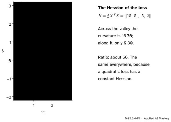
The running loss is a valley. Across the valley the walls are steep; along the floor the ground is almost level. The Hessian’s two eigen-directions point across and along, and its two eigenvalues say how sharply the loss curves each way.
M05.5.4-F1
The running loss is steep across its valley and nearly flat along it: curvatures 16.70 and 0.30.
A ratio of about 56 between the two curvatures has consequences. A step size that is safe across the valley crawls along it; a step size that moves briskly along it overshoots across. Newton’s method avoids the dilemma by dividing each direction by its own curvature.
Build it up
Step 1. One example at a time. The loss is the mean of the squared residuals \({(w x_i + b - y_i)^2}\). Write \({\tilde{\vect{x}}_i = (x_i, 1)}\) for example \(i\)’s row of the design matrix, so that its prediction is \({\tilde{\vect{x}}_i\T \vect{w}}\) with \({\vect{w} = (w, b)}\). Example \(i\)’s share of the loss, \({\tfrac1n (\tilde{\vect{x}}_i\T \vect{w} - y_i)^2}\), has gradient \({\tfrac2n (\tilde{\vect{x}}_i\T \vect{w} - y_i)\, \tilde{\vect{x}}_i}\) and Hessian \({\tfrac2n \tilde{\vect{x}}_i \tilde{\vect{x}}_i\T}\).
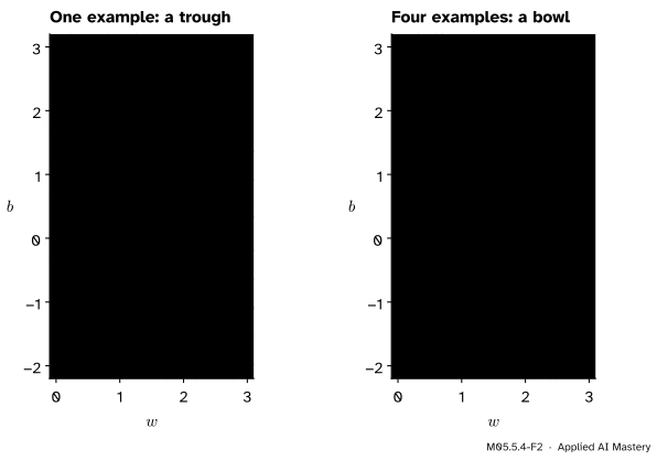
Step 2. That Hessian is a trough. The matrix \({\tilde{\vect{x}}_i \tilde{\vect{x}}_i\T}\) has rank one. Along any \(\vect{v}\) with \({\tilde{\vect{x}}_i\T \vect{v} = 0}\), a change of weights that leaves example \(i\)’s prediction unchanged, its curvature is zero.
M05.5.4-F2
One example’s squared error curves only across its own line of perfect fit. Four examples with different inputs curve in every direction: their troughs add up to a bowl.
Step 3. Add the examples. Summing over the four examples,
The curvature along \(\vect{v}\) is \({2/n}\) times the squared change of all the predictions. It is zero only if moving along \(\vect{v}\) changes no prediction, which needs dependent columns in \(\mat{X}\). So the mean squared error is a bowl or a trough, never a saddle: it is convex (M08.2).
The formal statement
The mean squared error. With \({L(\vect{w}) = \tfrac1n \norm{\mat{X}\vect{w} - \vect{y}}^2}\), the gradient of M05.2.3 is \({\nabla L(\vect{w}) = \tfrac2n \mat{X}\T (\mat{X}\vect{w} - \vect{y})}\). It is affine in \(\vect{w}\): \({\nabla L(\vect{w} + \vect{h}) = \nabla L(\vect{w}) + \tfrac2n \mat{X}\T\mat{X}\, \vect{h}}\), so its Jacobian, the Hessian, is the constant \({\tfrac2n \mat{X}\T\mat{X}}\).
The mean log loss. For logistic regression \({p_i = \sigma(\tilde{\vect{x}}_i\T \vect{w})}\) and
whose gradient (M05.2.3) has entries \({\pd{L}{w_j} = \tfrac1n \sum_i (p_i - y_i)\, x_{ij}}\). Only \(p_i\) depends on the weights, and by \({\sigma' = \sigma(1 - \sigma)}\) (M04.3.3) \({\pd{p_i}{w_k} = p_i(1 - p_i)\, x_{ik}}\). So
The weights \({p_i(1 - p_i)}\) lie between 0 and \({\tfrac14}\), so \({\vect{v}\T \mat{H}\vect{v} = \tfrac1n \sum_i p_i(1 - p_i)(\tilde{\vect{x}}_i\T \vect{v})^2 \ge 0}\): positive semidefinite again, but now it changes with \(\vect{w}\). The labels \(y_i\) do not appear in it at all.
The Newton step. Minimise the Taylor model \({q(\vect{h}) = L + \nabla L\T \vect{h} + \tfrac12 \vect{h}\T \mat{H}\vect{h}}\) over \(\vect{h}\). Its gradient in \(\vect{h}\) is \({\nabla L + \mat{H}\vect{h}}\); setting it to zero,
\[
\vect{h}_{\text{Newton}} = -\mat{H}^{-1} \nabla L ,
\]
the unique minimiser when \(\mat{H}\) is positive definite. When \(L\) is itself quadratic the model is exact, so the Newton step lands on the minimum. Methods built on it are M08.5.
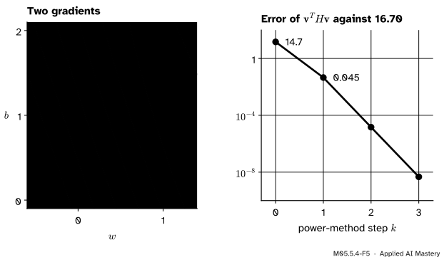
Curvature without the matrix. A model with a million weights has a Hessian with \({10^{12}}\) entries. But the gradient’s linear approximation gives a Hessian-vector product from two gradients,
exact for a quadratic. Feed it to the power method of M03.2.4, \({\vect{v} \leftarrow \mat{H}\vect{v} / \norm{\mat{H}\vect{v}}}\), and \({\vect{v}\T \mat{H}\vect{v}}\) converges to the largest eigenvalue \({\lambda_{\max}}\), provided the start is not perpendicular to its eigenvector. (The power method finds the eigenvalue of largest size; for these losses no eigenvalue is negative, so that is \({\lambda_{\max}}\).)
M05.5.4-F5
Left: two gradients a step \(\epsilon\) either side give \({\mat{H}\vect{v}}\) without forming \(\mat{H}\). Right: the power method built on such products finds the sharpness 16.70 in a few steps.
Why \({\lambda_{\max}}\) caps the learning rate. On a quadratic loss \({\nabla L(\vect{w}) = \mat{H}(\vect{w} - \vect{w}^*)}\), so a gradient step \({\vect{w}_{t+1} = \vect{w}_t - \eta \nabla L(\vect{w}_t)}\) moves the error \({\vect{e}_t = \vect{w}_t - \vect{w}^*}\) as
Along eigenvector \(\vect{q}_i\) the error is multiplied by \({1 - \eta\lambda_i}\) at every step. It shrinks in every direction exactly when \({\abs{1 - \eta \lambda_i} < 1}\) for all \(i\), that is when \({0 < \eta < 2/\lambda_{\max}}\) (M03.8.4). For the running loss \({2/16.70 \approx 0.1198}\).
Frontier note: the edge of stability
Cohen and co-authors (ICLR 2021) measured the sharpness \({\lambda_{\max}}\) of the training loss while training neural networks by full-batch gradient descent with step size \(\eta\). Their finding, in the words of their abstract: the sharpness “hovers just above” \({2/\eta}\). Training does not stay in the region where the quadratic analysis above promises stability: the loss behaves non-monotonically over short timescales, yet keeps decreasing over long ones. Measuring the sharpness of a large network is itself a job for Hessian-vector products, since the matrix is far too big to form.
Worked example
One Newton step from the origin on the running loss.
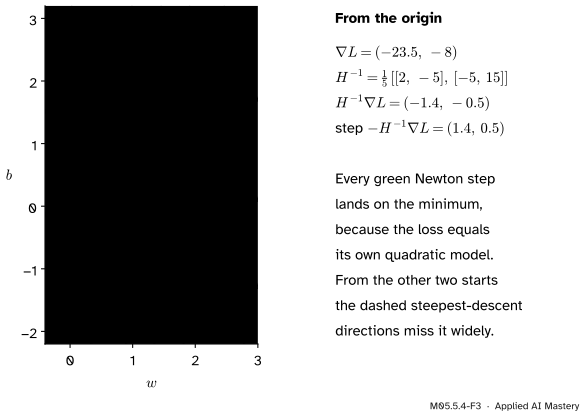
Gradient. At the origin only the constants of \({(15w + 5b - 23.5,\; 5w + 2b - 8)}\) remain: \({\nabla L(0, 0) = (-23.5, -8)}\).
Inverse Hessian.\({\det \mat{H} = 15 \times 2 - 5 \times 5 = 5}\), so swapping the diagonal and negating the off-diagonal gives
Step.\({-\mat{H}^{-1}\nabla L = (1.4, 0.5)}\), so the new point is \({(0, 0) + (1.4, 0.5) = (1.4, 0.5)}\): the least-squares line, in one step. From \({(2.5, -1.5)}\), where \({\nabla L = (6.5, 1.5)}\), the same calculation gives the step \({(-1.1, 2)}\), and again \({(2.5 - 1.1,\; -1.5 + 2) = (1.4, 0.5)}\).
M05.5.4-F3
Every Newton step lands on the minimum, because the loss equals its own quadratic model. The steepest-descent directions miss it, by far from two of the three starts.
Compare gradient descent. With \({\eta = 0.1}\) the first step from the origin is \({-0.1\,(-23.5, -8) = (2.35, 0.8)}\), which overshoots in \(w\); reaching the minimum takes many steps, because along the valley the error shrinks only by the factor \({1 - 0.1 \times 0.299 \approx 0.97}\) per step.
Code
The Hessian of the mean squared error from the design matrix, its eigenvalues and the largest stable learning rate:
Newton steps from three starts, and a Hessian-vector product fed to the power method. The product uses only the gradient function.
starts = [np.array([0.0, 0.0]), np.array([2.5, -1.5]), np.array([0.3, 2.6])]landed = [w - np.linalg.solve(H, grad_mse(w)) for w in starts]print("Newton lands at", [p.round(6).tolist() for p in landed])def hvp(w, v, eps=1e-3):return (grad_mse(w + eps * v) - grad_mse(w - eps * v)) / (2* eps)v = np.array([0.0, 1.0])for k inrange(20): hv = hvp(np.zeros(2), v) v = hv / np.linalg.norm(hv)sharpness = v @ hvp(np.zeros(2), v)print("power method:", round(sharpness, 4), " eigvalsh:", round(lam[1], 4))
Newton lands at [[1.4, 0.5], [1.4, 0.5], [1.4, 0.5]]
power method: 16.7006  eigvalsh: 16.7006
Gradient descent just below and just above \({2/\lambda_{\max}}\), from the start of the pitfall figure:
def descend(eta, steps, w=(0.3, 2.2)): w = np.array(w, dtype=float)for _ inrange(steps): w = w - eta * grad_mse(w)return np.linalg.norm(w - [1.4, 0.5])for eta in (0.10, 0.11, 0.13):print(f"eta = {eta}: distance after 12 steps {descend(eta, 12):.3f}, after 200 steps {descend(eta, 200):.2e}")
eta = 0.1: distance after 12 steps 1.364, after 200 steps 4.50e-03
eta = 0.11: distance after 12 steps 1.315, after 200 steps 2.42e-03
eta = 0.13: distance after 12 steps 3.506, after 200 steps 2.58e+13
Finally the log loss, with invented labels \({y = (0, 0, 1, 1)}\) on the same inputs: the formula \({\tfrac1n \mat{X}\T\mat{S}\mat{X}}\) against central differences of the gradient.
labels = np.array([0.0, 0.0, 1.0, 1.0])sigmoid =lambda z: 1/ (1+ np.exp(-z))def grad_log(w):return X.T @ (sigmoid(X @ w) - labels) / ndef hess_log(w): p = sigmoid(X @ w)return X.T @ np.diag(p * (1- p)) @ X / nfor w in (np.zeros(2), np.array([1.0, -2.5])): fd = np.column_stack([(grad_log(w + e) - grad_log(w - e)) /2e-5for e in1e-5* np.eye(2)])print(w, hess_log(w).round(4).tolist(), " eigenvalues", np.linalg.eigvalsh(hess_log(w)).round(4)," largest gap to differences", f"{np.abs(fd - hess_log(w)).max():.0e}")
[0. 0.] [[1.875, 0.625], [0.625, 0.25]]  eigenvalues [0.0374 2.0876]  largest gap to differences 2e-10
[ 1.  -2.5] [[1.3976, 0.4802], [0.4802, 0.1921]]  eigenvalues [0.0242 1.5655]  largest gap to differences 2e-11
At \({\vect{w} = \vect{0}}\) every \({p_i = \tfrac12}\), so \({\mat{S} = \tfrac14 \mat{I}}\) and the log loss’s Hessian is \({\tfrac1{16}\mat{X}\T\mat{X}}\), which is \({[[1.875, 0.625], [0.625, 0.25]]}\): one eighth of the mean squared error’s.
Explore
The curvature viewer in lesson M05.5.2 shows curvature at any point. On the running bowl the eigenvalues 2 and 4 never change as you drag the point; on Rosenbrock they change everywhere, which is why one Newton step is not enough there.
Pitfalls
M05.5.4-F4
Wrong beside right. Just above \({2/\lambda_{\max} \approx 0.12}\) the steps across the valley grow at every step; just below it they die away.
“A learning rate is fine as long as it is small compared with the gradient.”
What matters is the learning rate times the curvature. Across the running loss’s valley each step multiplies the error by \({1 - 16.70\,\eta}\): for \({\eta = 0.13}\) that is about \(-1.17\), so the error flips sign and grows by 17 per cent every step. The safe range is set by the sharpest direction, \({\eta < 2/\lambda_{\max}}\), whatever the size of the gradient.
“Just below \({2/\lambda_{\max}}\) is the best learning rate.”
It keeps the steep direction stable, but along the flat direction the error then shrinks only by \({1 - 0.1198 \times 0.299 \approx 0.964}\) per step. With a condition number of about 56, one fixed learning rate cannot suit both directions; that is the cost of ill-conditioning (M03.8.4), and the reason for Newton-like and adaptive methods (M08.4, M08.5).
“The Newton step always goes downhill.”
Only when \(\mat{H}\) is positive definite. On the saddle \({x^2 - y^2}\) the Newton step from any point jumps to the critical point at the origin, because the model’s only flat point is there. From \({(0.5, 1)}\), where \({f = -0.75}\), it lands at the origin, where \({f = 0}\): uphill. Practical methods check the curvature first (M08.5).
Check yourself
Recall
1. What is the Hessian of the mean squared error \({\tfrac1n \norm{\mat{X}\vect{w} - \vect{y}}^2}\), and its value for the running points?
Show answer
\({\tfrac2n \mat{X}\T\mat{X}}\), the same at every \(\vect{w}\); for the running points \({[[15, 5], [5, 2]]}\).
2. Why is that Hessian never negative in any direction?
Show answer
\({\vect{v}\T \mat{H}\vect{v} = \tfrac2n \norm{\mat{X}\vect{v}}^2 \ge 0}\): the curvature along \(\vect{v}\) is the squared change of the predictions.
3. What is the Hessian of the mean log loss of logistic regression?
Show answer
\({\tfrac1n \mat{X}\T\mat{S}\mat{X}}\) with \({\mat{S} = \operatorname{diag}(p_i(1 - p_i))}\). It depends on the weights through the \(p_i\) but not on the labels.
4. What is the Newton step, and why does one step solve least squares?
Show answer
\({-\mat{H}^{-1}\nabla L}\), the minimiser of the quadratic Taylor model. The mean squared error is quadratic, so it equals its model and the model’s minimiser is the true minimiser.
5. For which learning rates does gradient descent on a quadratic loss converge, and what is the limit for the running loss?
Show answer
For \({0 < \eta < 2/\lambda_{\max}}\). For the running loss \({2/16.70 \approx 0.12}\).
Exercises
1.★ A line is fitted by mean squared error to three points with inputs \({x = 0, 1, 2}\). Find the Hessian of the loss in \({(w, b)}\) and the largest stable learning rate.
Show solution
\({\mat{X}\T\mat{X} = \begin{bmatrix} \sum x_i^2 & \sum x_i \\ \sum x_i & n \end{bmatrix} = \begin{bmatrix} 5 & 3 \\ 3 & 3 \end{bmatrix}}\), so \({\mat{H} = \tfrac23 \mat{X}\T\mat{X} = \begin{bmatrix} 10/3 & 2 \\ 2 & 2 \end{bmatrix}}\), whatever the targets. Its trace is \({16/3}\) and determinant \({20/3 - 4 = 8/3}\), so
and the largest stable learning rate is \({2/4.775 \approx 0.419}\).
2.★★ Take one Newton step on the running loss from \({(2.5, -1.5)}\) by hand.
Show solution
The gradient \({(15w + 5b - 23.5,\; 5w + 2b - 8)}\) at \({(2.5, -1.5)}\) has first entry \(37.5 - 7.5 - 23.5 = 6.5\) and second entry \(12.5 - 3 - 8 = 1.5\).
With \({\mat{H}^{-1} = \tfrac15 [[2, -5], [-5, 15]]}\) the first entry of \({\mat{H}^{-1}\nabla L}\) is \({\tfrac15 (13 - 7.5)} = 1.1\) and the second is \({\tfrac15 (-32.5 + 22.5)} = -2\).
The new point is \({(2.5 - 1.1,\; -1.5 + 2) = (1.4, 0.5)}\).
3.★★★ Show that for every \(\vect{w}\) and \(\vect{v}\) the log loss’s curvature is at most one eighth of the mean squared error’s on the same inputs, and that the bound is reached at \({\vect{w} = \vect{0}}\). What is the log loss’s largest curvature for the running inputs?
Show solution
For the log loss \({\vect{v}\T\mat{H}\vect{v} = \tfrac1n \sum_i p_i(1 - p_i)(\tilde{\vect{x}}_i\T\vect{v})^2}\). Since \({p(1 - p) \le \tfrac14}\) for every \(p\) (the parabola peaks at \({p = \tfrac12}\)),
and the right side is one eighth of the mean squared error’s curvature. At \({\vect{w} = \vect{0}}\) every \({p_i = \tfrac12}\), so equality holds for every \(\vect{v}\). The largest curvature is then \({16.70 / 8 \approx 2.09}\), and no point has a larger one.
Summary card
A loss’s Hessian sets its shape, its Newton step and its learning rate.
M05.5.4-F1
Steep across, flat along.
Least squares.\({\mat{H} = \tfrac2n \mat{X}\T\mat{X}}\), constant and positive semidefinite.
Newton.\({\vect{h} = -\mat{H}^{-1}\nabla L}\): one step for a quadratic.
Sharpness.\({\lambda_{\max}}\) by power iteration on \({\mat{H}\vect{v}}\); stable if \({\eta < 2/\lambda_{\max}}\).
Sources and next steps
Sources. Each was opened and checked against this lesson on 15 November 2026.
Marc Peter Deisenroth, A. Aldo Faisal and Cheng Soon Ong, Mathematics for Machine Learning, Section 9.2.1, the remark after equation (9.12c): the Hessian of the least-squares objective is \({\mat{X}\T\mat{X}}\) (their objective has a different constant factor), positive definite when \(\mat{X}\) has full column rank, so the stationary point is a global minimum.
Andrew Ng and Tengyu Ma, CS229 Lecture Notes, Stanford, Section 2.4: Newton’s method \({\theta := \theta - \mat{H}^{-1}\nabla_\theta \ell(\theta)}\) with the Hessian of second partial derivatives, applied to logistic regression.
Alan Edelman and Steven G. Johnson, Matrix Calculus for Machine Learning and Beyond, Section 12.4.1 (minimising the quadratic model is the Newton step \({-\mat{H}^{-1}\nabla f}\)) and Section 12.4.2 (Hessian-vector products without forming \(\mat{H}\)).
Next. Module M05.6, Multiple integrals and change of variables, turns from derivatives to integrals over regions of the plane. Curvature returns in course M08: step sizes in M08.3 and Newton and quasi-Newton methods in M08.5.