Value, gradient and Hessian together give the best quadratic approximation of a smooth function near a point. Derive it from the one-variable Taylor polynomial of a slice, see its error shrink like the cube of the step, and read the curvature in every direction off the Hessian’s eigenvalues.
M05.5.2L2 Intermediate25 minIn review (what this means)
The maths and code on this page are checked by automated tests on every change, but an independent reader has not signed it off yet. Spot a mistake or a confusing step? Tell us.
Derive the second-order Taylor model f(a + h) ≈ f(a) + ∇f(a)ᵀh + (1/2) hᵀHh from the one-variable Taylor polynomial of the slice g(t) = f(a + t h).
Use the model to predict a change of f, and explain why it is exact for a quadratic and has an error of order ‖h‖³ otherwise.
Compute the curvature uᵀHu along a unit direction and show that it lies between the smallest and the largest eigenvalue of H.
Measure the model’s error against the step length on a log scale and read off the slope 3.
The question
On the running bowl, the step \({(0.1, 0.1)}\) from \({(1, 1)}\) changes \(f\) by 0.63, while the gradient’s linear model predicts 0.6. Which single extra term closes that gap of 0.03, and how good is the repaired model on a function that is not a bowl, such as Rosenbrock’s valley, whose curvature differs about 2500-fold from one direction to another? Every optimiser picks its next step by trusting some local model of the loss, so the quality of that model is the quality of the step.
From the last lesson
1. The Hessian is the Jacobian of which map, and what does \({\mat{H}\vect{h}}\) approximate?
Show answer
Of the gradient map. \({\mat{H}\vect{h}}\) approximates the change of the gradient, \({\nabla f(\vect{a} + \vect{h}) - \nabla f(\vect{a})}\).
2. What are the Hessians of the running bowl and of the running loss?
Show answer
\({\operatorname{diag}(2, 4)}\) and \({\begin{bmatrix} 15 & 5 \\ 5 & 2 \end{bmatrix}}\), the same at every point.
Intuition
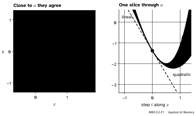
Zoom in on a smooth function near a point \(\vect{a}\) and three things describe it: its height, its tilt (the gradient) and its bend (the Hessian). The second-order Taylor model uses all three. It is a quadratic, so its contour lines are ellipses or hyperbolas, and close to \(\vect{a}\) it is almost indistinguishable from the function.
M05.5.2-F1
The cubic \({x^3 - 3x + y^2}\) near \({\vect{a} = (0.5, 0)}\). Close to \(\vect{a}\) the model’s dashed contour lines lie on the function’s solid ones. Along the slice the tangent line soon misses, the parabola hugs the curve much longer, and the gap that remains is exactly \(t^3\).
For this cubic, \({f(\vect{a}) = -1.375}\), the gradient \({(3x^2 - 3,\; 2y)}\) is \({(-2.25, 0)}\), and the Hessian \({\operatorname{diag}(6x, 2)}\) is \({\operatorname{diag}(3, 2)}\). The tangent line follows the slope alone. The parabola adds the bend, and the only thing it cannot follow is the cubic term.
Build it up
Step 1. Reduce to one variable. Fix a step \(\vect{h}\) and look along it: the slice \({g(t) = f(\vect{a} + t\vect{h})}\) of M05.1.3 is an ordinary function of \(t\), with \({g(0) = f(\vect{a})}\) and \({g(1) = f(\vect{a} + \vect{h})}\).
Step 2. Use the one-variable Taylor polynomial. By M04.8.3,
All that is left is to find \({g'(0)}\) and \({g''(0)}\) in terms of \(f\).
Step 3. The first derivative. Input \(i\) of \(f\) is \({a_i + t h_i}\), which changes at rate \(h_i\). The chain rule of M05.4.2 adds one product per input:
Step 4. The second derivative. Each \({\pd{f}{x_i}(\vect{a} + t\vect{h})}\) is again a function of \(t\), and the same chain rule gives its derivative as \({\sum_j h_j\, \frac{\partial^2 f}{\partial x_j \partial x_i}}\). So
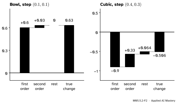
Step 5. Put it together at \({t = 0}\). On the running bowl at \({\vect{a} = (1, 1)}\) with \({\vect{h} = (0.1, 0.1)}\): the gradient term is \({(2, 4) \cdot (0.1, 0.1) = 0.6}\) and the curvature term is \({\tfrac12 (2 \times 0.01 + 4 \times 0.01) = 0.03}\). Together \({3 + 0.6 + 0.03 = 3.63}\), which is exactly \({f(1.1, 1.1) = 1.21 + 2.42}\).
M05.5.2-F2
The change of \(f\) split into its parts. For the bowl the gradient and curvature terms account for everything. For the cubic a remainder of \({0.4^3 = 0.064}\) is left over.
The formal statement
NoteTheorem: the second-order Taylor model
Let \({f : \R^n \to \R}\) have continuous second partial derivatives near \(\vect{a}\). Then
where the remainder satisfies \({r(\vect{h}) / \norm{\vect{h}}^2 \to 0}\) as \({\vect{h} \to \vect{0}}\). If the third partial derivatives are also continuous, there is a constant \(C\) with \({\abs{r(\vect{h})} \le C \norm{\vect{h}}^3}\) for all small \(\vect{h}\).
The first three terms are the second-order Taylor model: the gradient term is the linear model of M05.2.2 and the curvature term is the new part. The remainder is what the model misses.
Why the remainder is small. The one-variable Taylor theorem with remainder (M04.8.4) gives \({g(1) = g(0) + g'(0) + \tfrac12 g''(\tau)}\) for some \(\tau\) between 0 and 1. By Step 4,
with \({\mat{B} = \mat{H}(\vect{a} + \tau\vect{h}) - \mat{H}(\vect{a})}\). Each product \({h_i h_j}\) is at most \({\norm{\vect{h}}^2}\) in size, and each entry of \(\mat{B}\) tends to 0 as \({\vect{h} \to \vect{0}}\) because the second partial derivatives are continuous. So \({r(\vect{h}) / \norm{\vect{h}}^2 \to 0}\).
Why the cube. One order higher, the same theorem gives
for some \(\tau\) between 0 and 1. Differentiating Step 4 once more, \({g'''}\) is a sum of third partial derivatives each multiplied by three entries of \(\vect{h}\). Near \(\vect{a}\) those partial derivatives are bounded, and each product of three entries is at most \({\norm{\vect{h}}^3}\), so \({\abs{r} \le C\norm{\vect{h}}^3}\).
Exact for quadratics. A quadratic has no third derivatives, so its remainder is zero: that is why the bowl’s 0.63 came out exactly. For the cubic \({x^3 - 3x + y^2}\) the expansion
shows that the model captures every term but the last, so the remainder is exactly \({h_1^3}\).
M05.5.2-F5
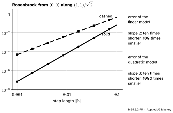
On a log scale the errors are straight lines. Shrink the step tenfold and the linear model’s error falls a hundredfold, the quadratic model’s a thousandfold.
Curvature along a direction. For a unit vector \(\vect{u}\), Step 4 at \({t = 0}\) says that the second derivative of the slice along \(\vect{u}\) is \({\vect{u}\T \mat{H} \vect{u}}\): the curvature of \(f\) along \(\vect{u}\) in this sense. Because \(\mat{H}\) is symmetric it has perpendicular unit eigenvectors \({\vect{q}_1, \vect{q}_2}\) with eigenvalues \({\lambda_1 \ge \lambda_2}\) (M03.3). Write \({\vect{u} = c_1 \vect{q}_1 + c_2 \vect{q}_2}\) with \({c_1^2 + c_2^2 = 1}\). Then
a weighted average of the eigenvalues. So \({\lambda_2 \le \vect{u}\T \mat{H} \vect{u} \le \lambda_1}\), with the extremes along the eigenvectors: this is the Rayleigh quotient of M03.3.4, and the same holds with \(n\) eigenvalues.
Worked example
Rosenbrock’s function near its minimum \({(1, 1)}\). There \({f = 0}\) and \({\nabla f = \vect{0}}\), and lesson M05.5.1 found the Hessian. So the model is the curvature term alone:
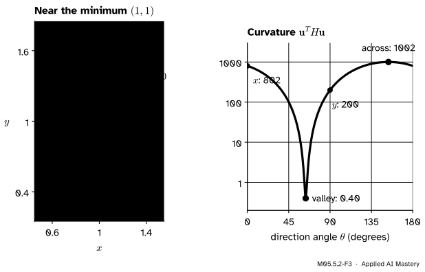
Curvature along the axes. Along \({(1, 0)}\) it is 802, along \({(0, 1)}\) it is 200.
Curvature along the valley. The valley floor is the parabola \({y = x^2}\), whose direction at \({(1, 1)}\) is \({(1, 2)}\). With \({\vect{u} = (1, 2)/\sqrt5}\),
The extremes. The trace is 1002 and the determinant \({802 \times 200 - 400^2 = 400}\), so the eigenvalues solve \({\lambda^2 - 1002\lambda + 400 = 0}\):
Their ratio is about 2508. The flattest direction is almost exactly the valley, whose curvature 0.4 is just above \({\lambda_2}\).
M05.5.2-F3
The quadratic model at \({(1, 1)}\) is a needle-thin bowl along the valley. Its curvature runs from 0.40 along the valley to 1002 across it, a factor of about 2500.
Testing the model. A step \({\vect{h} = (0.1, 0)}\) across the valley: the model predicts \({401 \times 0.01 = 4.01}\) and the truth is \({f(1.1, 1) = 0.01 + 100 \times 0.21^2 = 4.42}\). A step of the same length along the valley: the model predicts \({\tfrac12 \times 0.4 \times 0.01 = 0.002}\) and the truth is 0.0024. The model is good in both directions, but the same step length raises \(f\) about 1800 times more across the valley than along it: the trouble that gradient descent meets in M05.5.4.
Code
The model from scratch, tested on Rosenbrock from the origin along \({(1, 1)/\sqrt2}\), where neither the gradient nor the curvature term is zero.
import numpy as npdef rosen(p): x, y = preturn (1- x) **2+100* (y - x **2) **2def rosen_grad(p): x, y = preturn np.array([-2* (1- x) -400* x * (y - x **2), 200* (y - x **2)])def rosen_hess(p): x, y = preturn np.array([[2-400* y +1200* x **2, -400* x], [-400* x, 200.0]])def taylor2(f, grad, hess, a, h):"""Return the linear and the quadratic model's predictions of f(a + h).""" linear = f(a) + grad(a) @ hreturn linear, linear +0.5* h @ hess(a) @ ha, u = np.zeros(2), np.array([1.0, 1.0]) / np.sqrt(2)steps = [0.1, 0.01, 0.001]for t in steps: lin, quad = taylor2(rosen, rosen_grad, rosen_hess, a, t * u) true = rosen(a + t * u)print(f"t = {t:<6} linear error {abs(true - lin):.2e} quadratic error {abs(true - quad):.2e}")
t = 0.1     linear error 4.37e-01   quadratic error 6.82e-02
t = 0.01    linear error 4.98e-03   quadratic error 7.05e-05
t = 0.001   linear error 5.04e-05   quadratic error 7.07e-08
The slope on a log scale is the change in \({\log(\text{error})}\) per change in \({\log t}\):
def error(t): lin, quad = taylor2(rosen, rosen_grad, rosen_hess, a, t * u) true = rosen(a + t * u)returnabs(true - lin), abs(true - quad)slopes = [np.log10(error(1e-2)[k] / error(1e-3)[k]) for k in (0, 1)]print("linear model slope %.3f, quadratic model slope %.3f"%tuple(slopes))
linear model slope 1.995, quadratic model slope 2.999
The curvature in every direction at \({(1, 1)}\), by brute force over 3600 unit vectors, against the eigenvalues from numpy.linalg.eigvalsh (ascending order):
H = rosen_hess(np.array([1.0, 1.0]))angles = np.linspace(0, np.pi, 3600, endpoint=False)U = np.stack([np.cos(angles), np.sin(angles)]) # one unit vector per columncurvature = np.einsum("in,ij,jn->n", U, H, U)lam = np.linalg.eigvalsh(H)print("scan:", curvature.min().round(3), curvature.max().round(2))print("eigenvalues:", lam.round(3), " ratio", round(lam[1] / lam[0]))
scan: 0.399 1001.6
eigenvalues: [3.990000e-01 1.001601e+03]  ratio 2508
Explore
M05.5-X1
Curvature viewer
Drag the orange point, or set it with the sliders. Inside the dashed circle the solid lines are the function and the dashed lines its quadratic model at the same heights; the pale orange lines are the Hessian’s eigen-directions. Choose Rosenbrock, press To the critical point, and turn the wireframe: the model is a long, narrow bowl. Then visit the saddle and the monkey saddle.
Pitfalls
M05.5.2-F4
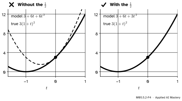
Wrong beside right. Without the one half the curvature term is doubled and the model bends away from the function immediately.
“The curvature term is \({\vect{h}\T \mat{H} \vect{h}}\).”
It is half of that. The one half comes from the one-variable Taylor polynomial, \({\tfrac12 g''(0)}\), just as \({x^2}\) has second derivative 2. Leave it out and the model’s curvature is doubled, as on the left of the figure. A quick check: the model of a quadratic must reproduce it exactly.
“The model is accurate, so I can trust it far from the point.”
The error grows like \({\norm{\vect{h}}^3}\). For the cubic it is exactly \({h_1^3}\): 0.064 for \({h_1 = 0.4}\) but 8 for \({h_1 = 2}\). Far out the model even changes character: at \({\vect{a} = (0.5, 0)}\) it is a bowl with a lowest point, while the cubic has no lowest point at all and falls without bound as \(x\) decreases. Optimisers that minimise a model therefore limit the step, with a line search or a trust region (M08.5).
“\({\vect{v}\T \mat{H} \vect{v}}\) is the curvature along \(\vect{v}\) for any vector.”
Only for a unit vector. For \({\vect{v} = 2\vect{u}}\) the value is four times larger. Divide by \({\vect{v}\T \vect{v}}\) first: that ratio is the Rayleigh quotient, and it depends only on the direction.
Check yourself
Recall
1. Write the second-order Taylor model of \(f\) at \(\vect{a}\) and name its terms.
Show answer
\({f(\vect{a}) + \nabla f(\vect{a})\T \vect{h} + \tfrac12 \vect{h}\T \mat{H}_f(\vect{a})\vect{h}}\): the value, the gradient term and the curvature term.
2. For the slice \({g(t) = f(\vect{a} + t\vect{h})}\), what are \({g'(0)}\) and \({g''(0)}\)?
Show answer
\({g'(0) = \nabla f(\vect{a})\T \vect{h}}\) and \({g''(0) = \vect{h}\T \mat{H}_f(\vect{a})\vect{h}}\).
3. When is the model exact, and how fast does its error shrink otherwise?
Show answer
It is exact for quadratics, which have no third derivatives. Otherwise, with continuous third partial derivatives, the error is at most \({C\norm{\vect{h}}^3}\): ten times shorter, a thousand times smaller.
4. Between which two numbers must the curvature \({\vect{u}\T \mat{H}\vect{u}}\) lie, and where are they reached?
Show answer
Between the smallest and the largest eigenvalue of \(\mat{H}\), reached along the corresponding eigenvectors.
5. What are the curvatures of Rosenbrock’s function at \({(1, 1)}\) along the valley and across it?
Show answer
About 0.40 along the valley and about 1002 across it, a ratio of about 2500.
Exercises
1.★ Find the second-order Taylor model of \({f(x, y) = x^2 y}\) at \({(1, 2)}\), use it to predict \({f(1.1, 1.9)}\), and compare with the true value.
Show solution
\({f(1, 2) = 2}\), \({\nabla f = (2xy,\; x^2) = (4, 1)}\) and \({\mat{H} = \begin{bmatrix} 2y & 2x \\ 2x & 0 \end{bmatrix} = \begin{bmatrix} 4 & 2 \\ 2 & 0 \end{bmatrix}}\). With \({\vect{h} = (0.1, -0.1)}\) the gradient term is \({0.4 - 0.1 = 0.3}\) and the curvature term is
The model predicts 2.3; the truth is \({1.21 \times 1.9 = 2.299}\). The remainder \({-0.001}\) is the cubic term \({h_1^2 h_2}\) of \({(1 + h_1)^2 (2 + h_2)}\).
2.★★ Use the model of the running loss at the origin to predict \({L(0.2, 0.1)}\). Why is the prediction exact?
Show solution
\({L(0, 0) = 18.5}\) and \({\nabla L(0, 0) = (-23.5, -8)}\), so the gradient term is \({-4.7 - 0.8 = -5.5}\). The curvature term is
The model gives \(18.5 - 5.5 + 0.41 = 13.41\), and direct substitution gives \(0.3 + 0.1 + 0.01 - 4.7 - 0.8 + 18.5 = 13.41\). It is exact because \(L\) is a quadratic.
3.★★★ For Rosenbrock’s Hessian at \({(1, 1)}\), find every unit direction whose curvature equals the average of the two eigenvalues, 501, and check one of them numerically.
Show solution
With \({\vect{u} = c_1\vect{q}_1 + c_2\vect{q}_2}\), the curvature is \({c_1^2\lambda_1 + c_2^2\lambda_2}\), which equals \({(\lambda_1 + \lambda_2)/2}\) exactly when \({c_1^2 = c_2^2 = \tfrac12}\): the directions at 45 degrees to both eigenvectors. The flat eigenvector points at about \({63.5}\) degrees, so the directions are at about \({18.5}\) and \({108.5}\) degrees (and their opposites). At \({18.5}\) degrees, \({\vect{u} \approx (0.948, 0.317)}\), and \({802\,u_1^2 - 800\,u_1 u_2 + 200\,u_2^2}\) comes to about \({721.3 - 240.7 + 20.1 = 500.7}\): 501 up to the rounding of the angle. Note that 501 is also the average of the axis curvatures 802 and 200, since both averages equal half the trace.
Summary card
Near a point, a smooth function is its value, plus a tilt, plus a bend.
Error. Zero for quadratics; at most \({C\norm{\vect{h}}^3}\) otherwise.
Curvature along a unit \(\vect{u}\).\({\vect{u}\T \mat{H}\vect{u}}\), between \({\lambda_{\min}}\) and \({\lambda_{\max}}\).
Rosenbrock at \({(1, 1)}\). Curvature from 0.40 to 1002.
Sources and next steps
Sources. Each was opened and checked against this lesson on 15 November 2026.
Marc Peter Deisenroth, A. Aldo Faisal and Cheng Soon Ong, Mathematics for Machine Learning, Section 5.8. Definitions 5.7 and 5.8 give the multivariate Taylor series and polynomial, and equation (5.158) writes the second-order term as \({\vect{\delta}\T \mat{H}\vect{\delta}}\), divided by \({2!}\) in the series (5.151). The book writes gradients as rows; this course writes them as columns, so its \({\nabla f\,\vect{\delta}}\) is our \({\nabla f\T \vect{h}}\).
Alan Edelman and Steven G. Johnson, Matrix Calculus for Machine Learning and Beyond, Section 12.1: the quadratic approximation of \(f\) by its value, gradient and Hessian, with an error that is small compared with the square of the step.
NumPy reference, numpy.linalg.eigvalsh: eigenvalues of a symmetric matrix in ascending order.
Next.M05.5.3 Minimum, maximum or saddle looks at the model where the gradient term vanishes, and lets the signs of the eigenvalues decide.