Do one map after another and the local linear maps compose too, so the Jacobian of the composite is the product of the Jacobians. Derive the general chain rule, check its shapes, and use it to differentiate a small neural network layer by layer.
M05.4.3L2 Intermediate25 minIn review (what this means)
The maths and code on this page are checked by automated tests on every change, but an independent reader has not signed it off yet. Spot a mistake or a confusing step? Tell us.
Derive the general chain rule J of f after g at a = J_f(g(a)) J_g(a) by composing two linear approximations.
Check the shapes of a Jacobian product and explain why the outer map’s Jacobian stands on the left.
Write the Jacobian of a dense layer and of an elementwise activation, and multiply them into the Jacobian of a 2-2-1 network by hand.
Verify a product of Jacobians against scipy.differentiate.jacobian of the composite map.
The question
A neural network is one simple map after another: a weighted sum, a squashing function, another weighted sum. Each piece has a Jacobian you can write down at a glance. What is the Jacobian of the whole network, and how do the pieces combine?
From the last lesson
1. State the chain rule for \({z = f(x, y)}\) when \(x\) and \(y\) both depend on \(s\) and \(t\).
Show answer
\({\pd{z}{s} = \pd{f}{x}\pd{x}{s} + \pd{f}{y}\pd{y}{s}}\), and the same with \(t\) in place of \(s\): one product per path, the paths added.
2. On the circle \({(\cos t, \sin t)}\), why is the answer \({-2\sin t\cos t}\) for the running bowl wrong?
Show answer
It keeps only the path through \(x\). Adding the path through \(y\), \({4\sin t\cos t}\), gives the true rate \({2\sin t\cos t}\).
Intuition
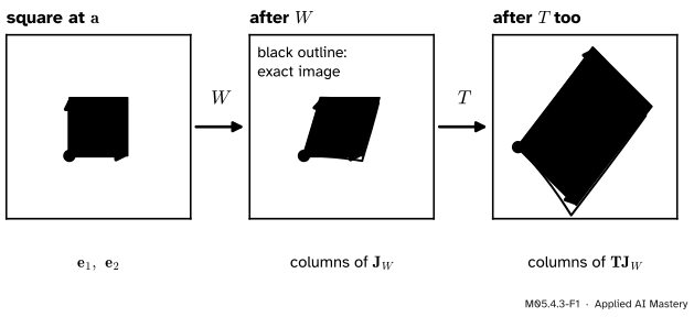
Send a small square through the running warp \(W\) and then through the linear map \(T\). The warp turns it into a near-parallelogram spanned by the columns of \({\mat{J}_W}\). Then \(T\), being linear, carries that parallelogram to another one, spanned by \(T\) applied to those columns.
M05.4.3-F1
A small square at \({\vect{a} = (\pi/2, 0)}\) through \(W\), then through \(T\). At each stage the image is close to the parallelogram of a matrix: first \({\mat{J}_W}\), then the product \({\mat{T}\mat{J}_W}\).
Linear maps compose by multiplying their matrices (M02.5). Near a point every smooth map is linear. So near a point, doing one map after another multiplies their Jacobians: the whole chain rule is that one sentence.
Build it up
Step 1. The first map, near \(\vect{a}\). For a small step \(\vect{h}\), \({g(\vect{a} + \vect{h}) \approx g(\vect{a}) + \mat{J}_g(\vect{a})\vect{h}}\). So the point \({\vect{b} = g(\vect{a})}\) moves by about \({\vect{k} = \mat{J}_g(\vect{a})\vect{h}}\).
Step 2. The second map, near \(\vect{b}\). For the small step \(\vect{k}\), \({f(\vect{b} + \vect{k}) \approx f(\vect{b}) + \mat{J}_f(\vect{b})\vect{k}}\). Note the point: \(f\) is linearised where it actually acts, at \({g(\vect{a})}\).
The matrix in front of \(\vect{h}\) is the Jacobian of the composite.
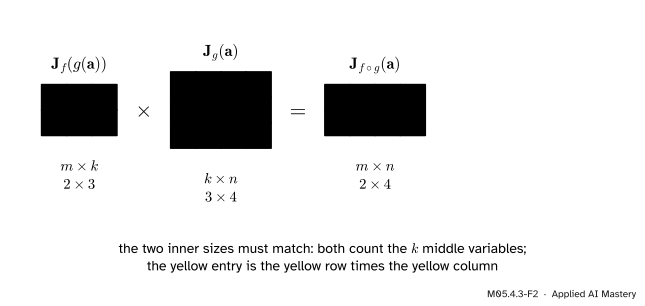
Step 4. Check the shapes. If \(g\) goes from \(\R^n\) to \(\R^k\) and \(f\) from \(\R^k\) to \(\R^m\), then \({\mat{J}_f}\) is \(m \times k\) and \({\mat{J}_g}\) is \(k \times n\). The inner sizes are both \(k\), the number of middle variables, and the product is \(m \times n\), as the composite needs.
M05.4.3-F2
The shape rule. The yellow entry of the product is the yellow row times the yellow column.
The formal statement
NoteThe general chain rule
Let \(g\) from \(\R^n\) to \(\R^k\) be differentiable at \(\vect{a}\), and \(f\) from \(\R^k\) to \(\R^m\) be differentiable at \({g(\vect{a})}\). Then \({f \circ g}\) is differentiable at \(\vect{a}\) and
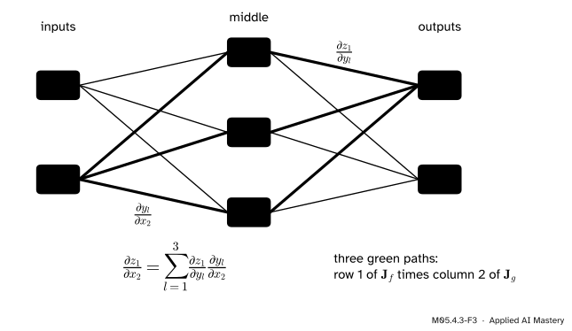
Entry by entry it is the path sum. Call the middle variables \({\vect{y} = g(\vect{x})}\). Row \(i\) of \({\mat{J}_f}\) times column \(j\) of \({\mat{J}_g}\) is
one term for each middle variable, a product of two branch derivatives. That is the tree rule of lesson M05.4.2, for every output and every input at once.
M05.4.3-F3
One entry of the product: the paths from one input to one output through every middle variable.
Go deeper: the proof, with the remainders
Write \({\vect{b} = g(\vect{a})}\), \({\vect{k} = g(\vect{a} + \vect{h}) - \vect{b}}\), \({\mat{A} = \mat{J}_g(\vect{a})}\) and \({\mat{B} = \mat{J}_f(\vect{b})}\). Differentiability gives \({\vect{k} = \mat{A}\vect{h} + r_g(\vect{h})}\) and \({f(\vect{b} + \vect{k}) = f(\vect{b}) + \mat{B}\vect{k} + r_f(\vect{k})}\). Substitute the first into the second:
We need the last two terms, divided by \({\norm{\vect{h}}}\), to tend to 0. Any matrix \(\mat{M}\) has a number \(C\) with \({\norm{\mat{M}\vect{v}} \le C\norm{\vect{v}}}\) for all \(\vect{v}\) (by Cauchy-Schwarz on each row, \(C\) can be the square root of the sum of the squared entries). So
The second factor is at most \({C_A + \norm{r_g(\vect{h})}/\norm{\vect{h}}}\), which stays bounded, and \({\vect{k} \to \vect{0}}\) as \({\vect{h} \to \vect{0}}\), so the first factor tends to 0. If \({\vect{k} = \vect{0}}\) the term is 0. Both remainders vanish faster than \(\vect{h}\), so \({\mat{B}\mat{A}}\) is the Jacobian of \({f \circ g}\). ∎
The Jacobians of a network’s pieces. A dense layer \({\vect{z} = \mat{W}\vect{x} + \vect{b}}\) has Jacobian \(\mat{W}\): the bias shifts every output but does not change how outputs respond to inputs. An elementwise activation \({a_i = \phi(z_i)}\) has \({\pd{a_i}{z_j} = \phi'(z_i)}\) when \({i = j}\) and 0 otherwise, because \(a_i\) does not depend on the other \(z_j\). Its Jacobian is the diagonal matrix \({\mathrm{diag}(\phi'(\vect{z}))}\); for tanh, \({\phi' = 1 - \tanh^2}\), so the diagonal is \({1 - a_i^2}\). A network is a composition of such pieces, so its input-output Jacobian is a product: the last layer’s on the left, the first layer’s on the right.
with \({\mat{D}^{(l)} = \mathrm{diag}(\phi'(\vect{z}^{(l)}))}\) evaluated at the values the forward pass produced. Its size is fixed by the ends alone: a network from 784 pixels to 10 scores has a \(10 \times 784\) Jacobian, however wide its hidden layers are. And because every factor can shrink or stretch the vectors it acts on, a long product can shrink or grow geometrically with depth, the vanishing and exploding gradients of M05.9.4 and DL02.4.
Frontier note: the same product in an autodiff library
Libraries compute these products without writing the matrices down. In JAX, jax.jacfwd(f)(x) and jax.jacrev(f)(x) return the full Jacobian of a function f, building it column by column or row by row; PyTorch offers torch.func.jacfwd and torch.func.jacrev. Shown here as text only: the course builds both modes from scratch in M05.8.
Worked example
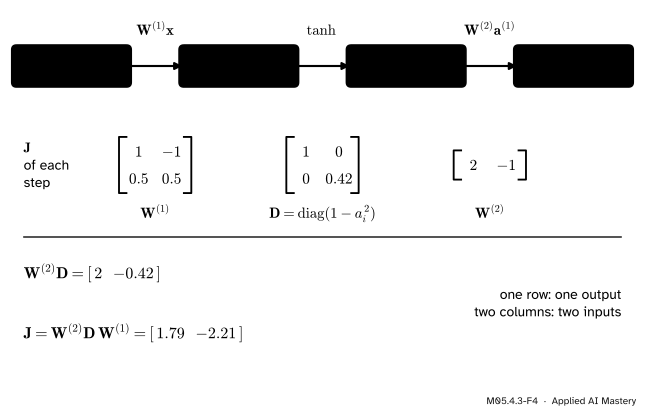
A 2-2-1 network by hand. Take \({\mat{W}^{(1)} = \begin{bmatrix} 1 & -1 \\ 0.5 & 0.5 \end{bmatrix}}\), then tanh, then \({\mat{W}^{(2)} = [\,2 \;\; {-1}\,]}\), with zero biases, at the input \({\vect{x} = (1, 1)}\).
Forward: \({\vect{z}^{(1)}} = {\mat{W}^{(1)}\vect{x}} = {(1 - 1,\; 0.5 + 0.5)} = {(0, 1)}\). Then \({\vect{a}^{(1)} = (\tanh 0, \tanh 1) \approx (0, 0.7616)}\), and the output is \({y = 2 \times 0 - 0.7616 = -0.7616}\).
The three Jacobians are \({\mat{W}^{(1)}}\), then \({\mat{D}} = {\mathrm{diag}(1 - 0^2,\; 1 - 0.7616^2)} \approx {\mathrm{diag}(1,\; 0.4200)}\), then \({\mat{W}^{(2)}}\). Multiply from the output end, so that every intermediate result is a single row:
One row for the one output, two columns for the two inputs: raising \(x_1\) by 0.01 raises the output by about 0.0179.
M05.4.3-F4
The worked example as a trace: forward values along the top, each step’s Jacobian beneath it, and their product, built from the output end.
The running chain of M04.3.4, read as Jacobians. There \({z = wx}\), \({p = \sigma(z)}\) and \({E = (p - y)^2}\), with \({w = 0.5}\), \({x = 2}\), \({y = 1}\). Each step has one input and one output, so each Jacobian is a \(1 \times 1\) matrix: \({dE/dp = 2(p - y) \approx -0.538}\), \({dp/dz = p(1 - p) \approx 0.197}\) and \({dz/dw = x = 2}\). Their product, about \(-0.212\), is the \({dE/dw}\) of M04.3.4. The one-variable chain rule is the case where every matrix is a single number.
Code
From scratch: the three layer Jacobians and their product, then SciPy on the composite. The network is written so that it accepts a batch of inputs along the first axis, as scipy.differentiate.jacobian requires.
import numpy as npfrom scipy.differentiate import jacobianW1 = np.array([[1.0, -1.0], [0.5, 0.5]])W2 = np.array([[2.0, -1.0]])def net(x): z = np.einsum("ij,j...->i...", W1, x) # works for one input or a batchreturn np.einsum("ij,j...->i...", W2, np.tanh(z))x0 = np.array([1.0, 1.0])a1 = np.tanh(W1 @ x0)D = np.diag(1- a1 **2)J_product = W2 @ D @ W1J_scipy = jacobian(net, x0).dfprint("a1 =", a1.round(4), " y =", net(x0).round(4))print("W2 D =", (W2 @ D).round(4), " product J =", J_product.round(4), " SciPy:", J_scipy.round(4))# The anchor picture: T after W at (pi/2, 0).T = np.array([[1.0, 1.0], [-1.0, 2.0]])warp =lambda v: np.array([v[0] +0.3* np.sin(v[1]), v[1] +0.3* np.sin(v[0])])tw =lambda v: np.einsum("ij,j...->i...", T, warp(v))a = np.array([np.pi /2, 0.0])J_warp = np.array([[1, 0.3* np.cos(a[1])], [0.3* np.cos(a[0]), 1]])print("T J_W =", (T @ J_warp).round(4).tolist(), " SciPy:", jacobian(tw, a).df.round(4).tolist())
The product and SciPy’s finite-difference Jacobian agree to the digits shown. Multiplying \({(\mat{W}^{(2)}\mat{D})\mat{W}^{(1)}}\) from the left only ever handles a single row; lesson M05.8.4 shows that this order is what makes reverse-mode differentiation, and backpropagation, cheap.
Explore
This module’s interactive, the grid warp, lives in lesson M05.4.1. Choose the running warp and set the point to \({x = 1.55}\), \({y = 0}\), next to \({(\pi/2, 0)}\): the read-out shows a Jacobian very close to the shear \({\begin{bmatrix} 1 & 0.3 \\ 0 & 1 \end{bmatrix}}\), with determinant close to 1. Then choose the linear map \(T\), whose Jacobian is \(T\) itself, with determinant 3. The anchor picture above applies \(T\) to the warp’s parallelogram, and exercise 3 below shows that the composite’s determinant is the product, 3.
Pitfalls
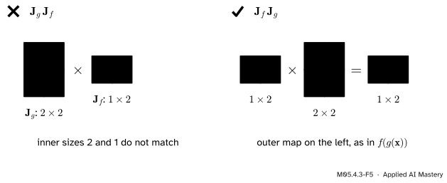
M05.4.3-F5
Wrong beside right, for \(g\) from \(\R^2\) to \(\R^2\) and \(f\) from \(\R^2\) to \(\R\). Inner first does not even fit; outer first gives the \(1 \times 2\) row of the composite.
“\(g\) acts first, so its Jacobian comes first: \({\mat{J}_g\mat{J}_f}\).”
The Jacobian of \({f \circ g}\) is written in the same order as \({f(g(\vect{x}))}\): the outer map on the left. The matrix that touches \(\vect{h}\) first is \({\mat{J}_g}\), on the right. In the wrong order the shapes often do not fit, and even when they do, as for two maps of the plane, matrices in general do not commute, so the answer is usually wrong.
“Evaluate both Jacobians at \(\vect{a}\).”
The outer Jacobian is evaluated at \({g(\vect{a})}\), the point where \(f\) actually acts. In the network, the tanh layer’s derivative uses \({\vect{z}^{(1)} = (0, 1)}\), the values it received, not the network’s input \({(1, 1)}\).
“The derivative of tanh at the layer’s output is \({1 - \tanh^2(a)}\).”
The derivative is \({\tanh'(z) = 1 - \tanh^2(z)}\), at the input \(z\). Because \({a = \tanh z}\), this equals \({1 - a^2}\), a formula in the output. Writing \({1 - \tanh^2(a)}\) applies tanh twice: for \({z = 1}\) it gives about 0.59 instead of 0.42. This exact bug is one that gradient checking catches (M05.9.3).
Check yourself
Recall
1. State the general chain rule for Jacobians.
Show answer
\({\mat{J}_{f \circ g}(\vect{a}) = \mat{J}_f(g(\vect{a}))\,\mat{J}_g(\vect{a})}\), with the outer Jacobian evaluated at \({g(\vect{a})}\).
2. For \(g\) from \(\R^n\) to \(\R^k\) and \(f\) from \(\R^k\) to \(\R^m\), what are the three shapes?
Show answer
\({\mat{J}_f}\) is \(m \times k\), \({\mat{J}_g}\) is \(k \times n\), and their product is \(m \times n\).
3. What is the Jacobian of a dense layer \({\mat{W}\vect{x} + \vect{b}}\)?
Show answer
\(\mat{W}\). The bias does not affect it.
4. What is the Jacobian of tanh applied to each entry of \(\vect{z}\)?
Show answer
The diagonal matrix with entries \({1 - \tanh^2(z_i)}\), that is \({1 - a_i^2}\).
5. How does one entry of a Jacobian product relate to the tree diagrams of M05.4.2?
Show answer
Entry \({(i, j)}\) is the sum over the middle variables of \({\pd{f_i}{y_l}\pd{y_l}{x_j}}\): one product per path from input \(j\) to output \(i\).
Exercises
1.★ A map \(g\) takes 5 numbers to 3 and \(f\) takes 3 numbers to 2. Give the shapes of \({\mat{J}_g}\), \({\mat{J}_f}\) and \({\mat{J}_{f \circ g}}\), and say which of the two products \({\mat{J}_f\mat{J}_g}\) and \({\mat{J}_g\mat{J}_f}\) is defined.
Show solution
\({\mat{J}_g}\) is \(3 \times 5\), \({\mat{J}_f}\) is \(2 \times 3\) and \({\mat{J}_{f \circ g}}\) is \(2 \times 5\). Only \({\mat{J}_f\mat{J}_g}\), a \((2 \times 3)(3 \times 5)\) product, is defined; \({\mat{J}_g\mat{J}_f}\) would need \(5 = 2\).
2.★★ Let \(g\) be the polar map and \(f\) the running bowl. Compute \({\mat{J}_f(g(\vect{a}))\,\mat{J}_g(\vect{a})}\) at \({\vect{a} = (2, \pi/6)}\) and compare with lesson M05.4.2.
Show solution
\({g(\vect{a}) = (\sqrt3, 1)}\), where \({\mat{J}_f = [\,2x \;\; 4y\,] = [\,2\sqrt3 \;\; 4\,]}\). Then
the two derivatives \({\pd{z}{r} = 5}\) and \({\pd{z}{\theta} = 2\sqrt3 \approx 3.46}\) found with the tree in M05.4.2.
3.★★★ For maps of the plane, show that \({\det\mat{J}_{f \circ g}(\vect{a}) = \det\mat{J}_f(g(\vect{a}))\,\det\mat{J}_g(\vect{a})}\), and check it for \(T\) after \(W\) at \({(\pi/2, 0)}\).
Show solution
By the chain rule the Jacobian of the composite is the product of the two Jacobians, and the determinant of a product of square matrices is the product of their determinants (M02.8). At \({(\pi/2, 0)}\), \({\det\mat{J}_W = 1 \times 1 - 0.3 \times 0 = 1}\) and \({\det\mat{T} = 2 + 1 = 3}\), so the composite has determinant 3. Directly, \({\mat{T}\mat{J}_W = \begin{bmatrix} 1 & 1.3 \\ -1 & 1.7 \end{bmatrix}}\) has determinant \({1.7 + 1.3 = 3}\). Normalising flows rely on this rule to add up the log-determinants of many layers.
Summary card
Near a point, composing maps multiplies their Jacobians.
Network: \({\mat{J} = \mat{W}^{(2)}\mat{D}\,\mat{W}^{(1)}}\), here \({[\,1.79 \;\; {-2.21}\,]}\).
Sources and next steps
Sources. Each was opened and checked against this lesson on 15 November 2026.
Paige Bright, Alan Edelman and Steven G. Johnson, Matrix Calculus (for Machine Learning and Beyond), notes for MIT 18.S096, Section 2.5: the chain rule as the product of the Jacobians, \({g'(h(x))\,h'(x)}\), and Example 15, the shapes \(m \times p\) times \(p \times n\) and why the reversed product does not even fit.
Marc Peter Deisenroth, A. Aldo Faisal and Cheng Soon Ong, Mathematics for Machine Learning, Section 5.2.2 (the chain rule as a matrix multiplication, Equation 5.53) and Section 5.6.1 (a deep network as a composition of layers, Equations 5.111 to 5.113).
Gilbert Strang and Edwin Herman, Calculus Volume 3 (OpenStax), Section 4.5, Theorem 4.10: the generalised chain rule, a sum over the intermediate variables, which is one entry of the product.