A polar cell has area r times dr times dtheta, so a disc is integrated with dA = r dr dtheta. That one factor r turns the Gaussian over the plane into an easy integral, 2 pi, and proves at last that the bell curve has area the square root of 2 pi.
M05.6.3L2 Intermediate25 minIn review (what this means)
The maths and code on this page are checked by automated tests on every change, but an independent reader has not signed it off yet. Spot a mistake or a confusing step? Tell us.
Derive the area of a polar cell from the area of a sector, and explain why dA = r dr dtheta.
Convert a double integral over a disc, a ring or a wedge to polar coordinates and evaluate it.
Prove that the integral of exp(−(x² + y²)/2) over the plane is 2 pi, and deduce that the bell curve has area the square root of 2 pi, justifying the step through squares and discs.
Compute a polar Riemann sum from scratch and check it against scipy.integrate.dblquad.
The question
The bell curve \({e^{-x^2/2}}\) has no antiderivative built from elementary functions (M04.7.4), yet every normal density carries the exact factor \({1/\sqrt{2\pi}}\) so that its area is 1. Lessons M04.7.3 and M06.6.4 promised a proof. Where does an exact \({\sqrt{2\pi}}\) come from, when no single-variable method can find it? This constant sits in every Gaussian likelihood that machine learning maximises.
From the last lesson
1. Write the triangle \({0 < y < x < 1}\) as a type II region.
Show answer
\({0 \le y \le 1}\) and \({y \le x \le 1}\).
2. How is the probability that \({(X, Y)}\) lands in a region \(D\) computed from a joint density \(p\)?
Show answer
As \({\iint_D p\,dA}\).
Intuition
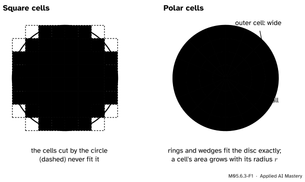
Square cells are made for rectangles. On a disc they leave a ragged edge of cells that are partly in and partly out. Cells cut along circles and rays, rings and wedges, fit a disc exactly.
M05.6.3-F1
Square cells (left) cannot follow a circle; polar cells (right) fit it exactly. But the polar cells are not all the same size: a cell at the rim is much wider than one near the centre.
That is the whole story of this lesson. Polar cells make round regions easy, as long as each cell is weighted by its true area. The cells in the same wedge all have the same angle and the same depth \({\Delta r}\), yet the outer ones are wider, in proportion to their distance \(r\) from the centre.
Build it up
Step 1. Polar coordinates. A point is \({(x, y) = (r\cos\theta,\; r\sin\theta)}\), with \({r \ge 0}\) its distance from the origin and \(\theta\) its angle (M01.5.2). A disc of radius \(a\) is simply \({0 \le r \le a}\), \({0 \le \theta \le 2\pi}\): a rectangle in \({(r, \theta)}\).
Step 2. One polar cell. Fix radii \(r\) and \({r + \Delta r}\) and angles \(\theta\) and \({\theta + \Delta\theta}\). The cell between them is a piece of a ring.
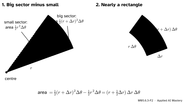
Step 3. Its area, exactly. A sector of radius \(\rho\) and angle \(\phi\) has area \({\tfrac12 \rho^2 \phi}\): lesson M04.1.2 found \({\phi/2}\) for the unit circle, with \(\phi\) in radians, and a radius \(\rho\) multiplies every area by \({\rho^2}\). The cell is a big sector minus a small one:
The bracket \({r + \tfrac12\Delta r}\) is the cell’s middle radius. So the area of a polar cell is its middle radius times \({\Delta r}\) times \({\Delta\theta}\), exactly.
M05.6.3-F2
The area of a polar cell. Subtracting two sectors leaves \({(r + \tfrac12\Delta r)\,\Delta r\,\Delta\theta}\): the cell is nearly a rectangle with sides \({\Delta r}\) and \({r\,\Delta\theta}\).
Step 4. A polar Riemann sum. Cut the \({(r, \theta)}\) rectangle into cells, evaluate \(f\) at each cell’s middle \({(r^*, \theta^*)}\), and add
This is an ordinary Riemann sum in \(r\) and \(\theta\) for the function \({f \cdot r}\). As the cells shrink it tends to an iterated integral in \(r\) and \(\theta\), with the extra factor \(r\).
The formal statement
NoteTheorem: double integrals in polar coordinates
If \(f\) is continuous on a region \(D\) described by \({\alpha \le \theta \le \beta}\) and \({r_1(\theta) \le r \le r_2(\theta)}\), with \({0 \le r_1 \le r_2}\) and \({\beta - \alpha \le 2\pi}\), then
Why (a sketch). Each polar sum of Step 4 is two things at once. It is a sum of value times true area over cells that tile \(D\) (exactly for a disc, a ring or a wedge; for other regions only the cells cut by the edge are left over, and they add nothing in the limit, as in M05.6.2). Cells of any shape work as well as rectangles once they all shrink, by the same uniform continuity as in M05.6.1, so the sum tends to \({\iint_D f\,dA}\). And it is a midpoint Riemann sum of \({f \cdot r}\) over a region of the \({(r, \theta)}\) plane, so it tends to the iterated integral (M05.6.2). Two limits of the same numbers are equal. Lesson M05.6.4 shows that the factor \(r\) is one case of a general rule.
The Gaussian over the plane. Integrate \({e^{-(x^2 + y^2)/2} = e^{-r^2/2}}\) over the disc of radius \(R\). The substitution \({u = r^2/2}\), \({du = r\,dr}\) (M04.7.1) is possible only because of the factor \(r\):
As \({R \to \infty}\) this tends to \({2\pi}\): the integral over the whole plane is \({2\pi}\).
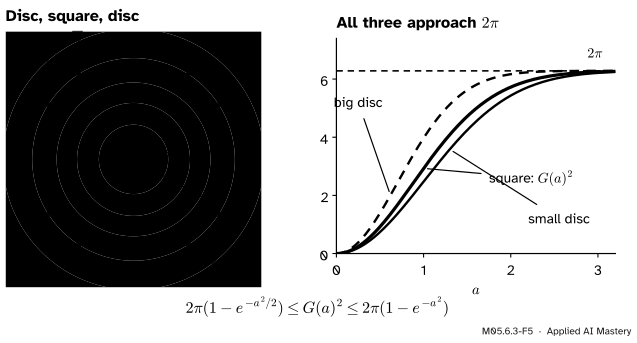
From the plane to the bell. Let \({G(a) = \int_{-a}^{a} e^{-x^2/2}\,dx}\). Over the square \({[-a, a]^2}\) the integrand factorises as \({e^{-x^2/2}\,e^{-y^2/2}}\), so by M05.6.1 the integral over the square is \({G(a)^2}\). The square contains the disc of radius \(a\) and sits inside the disc of radius \({a\sqrt2}\), and the integrand is positive, so
The squeeze. The integral over the square is trapped between the integrals over two discs, and both discs give \({2\pi}\) in the limit, so the square does too.
Both bounds tend to \({2\pi}\) as \({a \to \infty}\), so \({G(a)^2 \to 2\pi}\). The improper integral \({G = \lim G(a)}\) exists (M04.7.3), so \({G^2 = 2\pi}\), and since \({G > 0}\),
So the standard normal density \({\tfrac{1}{\sqrt{2\pi}} e^{-x^2/2}}\) has area exactly 1, as M06.6.4 needed. The squeeze is the step that justifies the trick: every integral in it is over a bounded square or disc, and the only limits taken are of ordinary numbers as \(a\) grows.
Frontier note: the (2 pi) to the power d/2 in every Gaussian likelihood
The same factorising works in any number of dimensions, one factor \({\sqrt{2\pi}}\) per coordinate:
That is the constant in front of the multivariate normal density (M07.3), and its logarithm, \({\tfrac{d}{2}\log 2\pi}\), is a constant term in the negative log-likelihood of every model with Gaussian noise. It does not depend on the parameters, so it drops out when the likelihood is maximised; for noise of fixed spread, what remains is the squared error.
Worked example
The area of a disc of radius \(a\). With \({f = 1}\), the inner integral is \({\int_0^a r\,dr = \tfrac{a^2}{2}}\), and the outer one multiplies by \({2\pi}\): the area is \({\pi a^2}\).
The running bowl over the unit disc. In polar form,
The disc has area \(\pi\), so the bowl’s average height over it is \({\tfrac34}\).
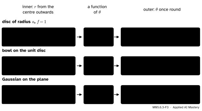
M05.6.3-F3
Three integrals over discs. In each row the factor \(r\) from \({dA = r\,dr\,d\theta}\) sits inside the first box.
Code
From scratch: a polar midpoint sum, each cell weighted by its middle radius.
import mathimport numpy as npdef polar_sum(f, R, n_r, n_theta):"""Midpoint sum of f(x, y) over the disc r <= R with n_r rings and n_theta wedges.""" dr, dth = R / n_r, 2* math.pi / n_theta r = dr * (np.arange(n_r) +0.5) # middle radii th = dth * (np.arange(n_theta) +0.5) # middle angles Rg, Tg = np.meshgrid(r, th)return np.sum(f(Rg * np.cos(Tg), Rg * np.sin(Tg)) * Rg) * dr * dth # note the factor rbowl =lambda x, y: x**2+2* y**2bell =lambda x, y: np.exp(-(x**2+ y**2) /2)print("disc area:", polar_sum(lambda x, y: np.ones_like(x), 1, 4, 16), " pi =", round(math.pi, 6))for n in [10, 20, 40, 80]:print(n, "rings: bowl", round(polar_sum(bowl, 1, n, 4* n), 5)," bell, R = 6:", round(polar_sum(bell, 6, n, 4* n), 5))
disc area: 3.141592653589793  pi = 3.141593
10 rings: bowl 2.34441   bell, R = 6: 6.38055
20 rings: bowl 2.35325   bell, R = 6: 6.30693
40 rings: bowl 2.35546   bell, R = 6: 6.28909
80 rings: bowl 2.35601   bell, R = 6: 6.28466
The disc’s area comes out as \(\pi\) exactly, for any number of cells, because each polar cell’s area is exactly its middle radius times \({\Delta r\,\Delta\theta}\). The bell’s sums approach \({2\pi \approx 6.2832}\), their error falling about fourfold each time the rings double.
The library, two ways. In polar form dblquad takes \(r\) as its inner variable; on growing squares it shows \({G(a)^2}\) climbing to \({2\pi}\), and quad gives the bell’s area directly.
from scipy.integrate import dblquad, quadpolar = dblquad(lambda r, th: math.exp(-r**2/2) * r, 0, 2* math.pi, 0, 10)[0]squares = {a: dblquad(lambda y, x: math.exp(-(x**2+ y**2) /2), -a, a, -a, a)[0] for a in (1, 2, 3, 6)}G = quad(lambda x: math.exp(-x**2/2), -math.inf, math.inf)[0]print("polar:", round(polar, 8), " 2 pi:", round(2* math.pi, 8))print({a: round(v, 4) for a, v in squares.items()})print("bell area:", round(G, 6), " sqrt(2 pi):", round(math.sqrt(2* math.pi), 6))
Choose a function, a region and a grid, then slide the number of cells. Put the disc under square cells and count the dashed cells at its edge; switch to polar cells and they vanish, while the yellow inner and outer cells show the factor \(r\) at work.
Pitfalls
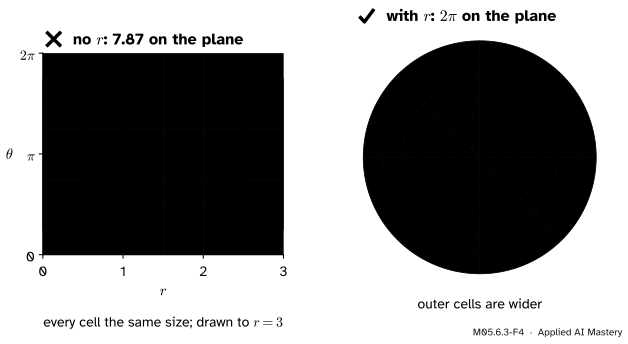
M05.6.3-F4
Wrong beside right, with the cells drawn out to \({r = 3}\). Without the factor \(r\), every cell of the \({(r, \theta)}\) rectangle counts the same; in the plane the outer cells are far larger. Over the whole plane the true integral is \({2\pi}\), not 7.87.
“Polar coordinates: replace \({dx\,dy}\) by \({dr\,d\theta}\).”
The cells of \({dr\,d\theta}\) are not the same size: their area is \({r\,dr\,d\theta}\). Dropping \(r\) gives \({\int_0^{2\pi}\int_0^\infty e^{-r^2/2}\,dr\,d\theta} = {2\pi\sqrt{\pi/2}} \approx 7.87\) instead of \({2\pi}\), and it loses the factor that made the substitution \({u = r^2/2}\) possible.
“Squaring an improper integral just splits it, so the proof is one line.”
The one-line version, \({G^2 = \iint_{\R^2} e^{-(x^2 + y^2)/2}\,dA}\), hides a step: an integral over the whole plane is a limit, and limits over squares and over discs need not agree in general. Here they do because the integrand is positive and the squeeze traps the squares between discs. Take that step out and the proof has a gap.
“Polar coordinates always make a double integral easier.”
Only when the region or the integrand is round. In polar form the unit square needs two pieces, \({r \le 1/\cos\theta}\) for \({\theta \le \pi/4}\) and \({r \le 1/\sin\theta}\) beyond, so Cartesian coordinates, with constant limits, are simpler there.
Check yourself
Recall
1. What is the exact area of the polar cell between radii \(r\) and \({r + \Delta r}\) and angles \(\theta\) and \({\theta + \Delta\theta}\)?
Show answer
\({\big(r + \tfrac12\Delta r\big)\,\Delta r\,\Delta\theta}\): its middle radius times \({\Delta r}\) times \({\Delta\theta}\).
2. What is \(dA\) in polar coordinates?
Show answer
\({dA = r\,dr\,d\theta}\).
3. What is the integral of \({e^{-(x^2 + y^2)/2}}\) over the disc of radius \(R\), and over the plane?
Show answer
\({2\pi(1 - e^{-R^2/2})}\), which tends to \({2\pi}\) over the whole plane.
4. Why does the integral over the square \({[-a, a]^2}\) equal \({G(a)^2}\)?
Show answer
Because \({e^{-(x^2 + y^2)/2}} = {e^{-x^2/2}\,e^{-y^2/2}}\) factorises, and over a rectangle the integral of a product \({g(x)h(y)}\) is the product of the two single integrals.
5. What is the area under the bell curve \({e^{-x^2/2}}\), and why is it the positive square root of \({2\pi}\)?
Show answer
\({\sqrt{2\pi} \approx 2.5066}\). Its square is \({2\pi}\), and the integral of a positive function is positive.
Exercises
1.★ Find the area of the ring \({1 \le r \le 2}\).
Show solution
\({\int_0^{2\pi} \int_1^2 r\,dr\,d\theta} = {2\pi \cdot \tfrac{4 - 1}{2}} = 3\pi\), which is \({\pi \cdot 2^2 - \pi \cdot 1^2}\).
2.★★ Compute \({\iint e^{-(x^2 + y^2)}\,dA}\) over the unit disc.
Show solution
In polar form the integrand is \({e^{-r^2}}\). With \({u = r^2}\), \({du = 2r\,dr}\): \({\int_0^1 e^{-r^2} r\,dr} = {\tfrac12\int_0^1 e^{-u}\,du} = {\tfrac{1 - e^{-1}}{2}}\). The outer integral multiplies by \({2\pi}\): \({\pi(1 - e^{-1}) \approx 1.986}\).
3.★★★ From \({\int_{-\infty}^{\infty} e^{-x^2/2}\,dx = \sqrt{2\pi}}\), find \({\int_{-\infty}^{\infty} e^{-x^2/(2\sigma^2)}\,dx}\) for \({\sigma > 0}\) and \({\int_0^\infty e^{-x^2}\,dx}\).
Show solution
For the first, substitute \({x = \sigma z}\), \({dx = \sigma\,dz}\): the integral becomes \({\sigma \int e^{-z^2/2}\,dz = \sigma\sqrt{2\pi}}\), the normaliser of a normal density with standard deviation \(\sigma\). For the second, substitute \({x = t/\sqrt2}\), \({dx = dt/\sqrt2}\): \({\int_0^\infty e^{-t^2/2}\,\tfrac{dt}{\sqrt2}}\). The bell is symmetric, so \({\int_0^\infty e^{-t^2/2}\,dt = \tfrac12\sqrt{2\pi}}\), and the answer is \({\tfrac{\sqrt{2\pi}}{2\sqrt2} = \tfrac{\sqrt\pi}{2} \approx 0.886}\).
Summary card
In polar coordinates, every cell is weighted by its radius: \({dA = r\,dr\,d\theta}\).
M05.6.3-F1
Polar cells fit discs and widen outwards.
Polar cell.\({\Delta A = (r + \tfrac12\Delta r)\,\Delta r\,\Delta\theta}\), exactly.
Theorem.\({\iint_D f\,dA} = {\int_\alpha^\beta \int_{r_1}^{r_2} f\,r\,dr\,d\theta}\), with \(f\) at \({(r\cos\theta, r\sin\theta)}\).
Disc and bowl. Area \({\pi a^2}\); the bowl over the unit disc gives \({3\pi/4}\).
Sources. Each was opened and checked against this lesson on 15 November 2026.
Gilbert Strang and Edwin Herman, Calculus Volume 3, Section 5.3, Double integrals in polar coordinates, OpenStax. The area of a polar rectangle as \({r^*\,\Delta r\,\Delta\theta}\) with \(r^*\) the middle radius, the double Riemann sum in polar form (equation 5.8), the iterated integral with \({r\,dr\,d\theta}\) over a general polar region (Theorem 5.8, equation 5.9), and Example 5.35, an integral of \({e^{-10(x^2 + y^2)}}\) over the whole plane by the same method.
SciPy reference, scipy.integrate.dblquad: the inner variable is the first argument of the integrand, here \(r\), with \(\theta\) outside.
Next.M05.6.4 Change of variables and the Jacobian determinant shows that the factor \(r\) is the Jacobian determinant of the polar map, and does the same for any smooth one-to-one map, including the maps that turn one probability density into another.