An area over an infinite range is the limit of areas over growing finite ranges. Find exactly when the area under 1/xᵖ is finite, see a spike with finite area, and check that a probability density has total area 1, with the mean of the exponential distribution found by parts.
Define an improper integral as a limit of ordinary integrals, both for an infinite range and for an integrand that blows up at an end.
Derive that the integral of 1/xᵖ from 1 to infinity converges exactly when p > 1, with value 1/(p - 1).
Show that a spike such as 1/sqrt(x) on (0, 1] can enclose a finite area.
Check that the exponential density has total area 1 and find its mean 1/lambda by integration by parts.
Compute improper integrals with scipy.integrate.quad and numpy.inf, and explain why a numerical answer alone cannot prove convergence.
In review. The maths and code on this page are checked by automated tests on every change, but an independent reader has not signed it off yet. Spot a mistake or a confusing step? Tell us.
The question
A probability density must enclose a total area of exactly 1. Yet the bell curve and the exponential curve never reach zero: their graphs run on for ever, to the right and, for the bell, to the left too. How can an area that never ends be 1? And why does the curve \({1/x}\), which also falls towards zero, enclose an infinite area instead?
From the last lesson
1. State the integration-by-parts formula in its short form.
Show answer
\({\int u\,dv = uv - \int v\,du}\).
2. In \({\int x\,e^x\,dx}\), which choice of \(u\) works, and what goes wrong with the other?
Show answer
\({u = x}\) and \({dv = e^x\,dx}\) works, leaving \({\int e^x\,dx}\). With \({u = e^x}\) the new integral is \({\int \frac{x^2}{2}e^x\,dx}\), harder than the original.
Intuition
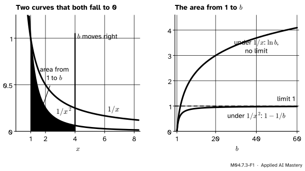
Put two curves side by side: \({1/x^2}\) and \({1/x}\), from \({x = 1}\) onwards. Both start at height 1 and both fall towards zero. Neither ever reaches it.
M04.7.3-F1
Two curves that look alike. Left: both fall to zero. Right: the area under each from 1 to a moving end \(b\). Under \({1/x^2}\) it settles on 1; under \({1/x}\) it climbs for ever, slowly but without bound.
You cannot shade an area that never ends, but you can shade the area from 1 to a finite end \(b\), and watch what happens as \(b\) moves right. The antiderivatives of M04.6.3 give it at once:
At \({b = 10, 100, 1000}\) the first is 0.9, 0.99, 0.999: it settles on 1. The second is about 2.30, 4.61, 6.91: it keeps growing, by the same \({\ln 10 \approx 2.30}\) for every tenfold step, and passes any number you name. The area out to infinity is what the area up to \(b\) settles on as \(b\) grows, if it settles at all. Under \({1/x^2}\) it does, at 1. Under \({1/x}\) it does not.
Build it up
Step 1. An infinite range. Define the area out to infinity as a limit (M04.1.3):
When the limit exists, the integral converges; when it does not, the integral diverges. So \({\int_1^\infty dx/x}\) diverges: \({\ln b}\) has no finite limit.
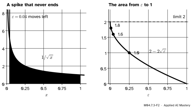
Step 2. A spike. The second kind of trouble is a graph that shoots up at one end. The function \({1/\sqrt{x}}\) is infinitely tall near \({x = 0}\). Stop a little short of the spike, at a small \({\varepsilon > 0}\), and let \(\varepsilon\) shrink:
A spike with a finite area. As the cut-off \(\varepsilon\) moves towards 0, the area from \(\varepsilon\) to 1 takes the values 1.0, 1.6 and 1.8 and closes in on 2, although the graph above it has no top.
At \({\varepsilon = 0.25}\), \({0.04}\) and \({0.01}\) the areas are 1.0, 1.6 and 1.8. An infinitely tall spike can stand on a finite area, because it is also infinitely thin. Not every spike does: for \({1/x}\) the same steps give \({\int_\varepsilon^1 dx/x = -\ln\varepsilon}\), which grows without bound.
Step 3. Both ends. For a range that is infinite at both ends, split it at any point \(c\) and require each half to converge on its own. The value then does not depend on \(c\).
The formal statement
NoteDefinition: improper integrals
If \(f\) is continuous on \({[a, \infty)}\), then \({\int_a^\infty f(x)\,dx}\) is \({\lim_{b \to \infty} \int_a^b f(x)\,dx}\).
If \(f\) is continuous on \({(a, b]}\) but unbounded near \(a\), then \({\int_a^b f(x)\,dx}\) is \({\lim_{\varepsilon \to 0^+} \int_{a + \varepsilon}^b f(x)\,dx}\).
\({\int_{-\infty}^{\infty} f}\) is \({\int_{-\infty}^{c} f + \int_{c}^{\infty} f}\), and both halves must converge.
The integral converges when the limit exists and is finite, and diverges otherwise. The ranges \({(-\infty, b]}\) and a spike at the right end are handled in the same way.
NoteResult: the area under \({1/x^p}\)
\({\int_1^\infty \dfrac{dx}{x^p}}\) converges exactly when \({p > 1}\), and then it equals \({\dfrac{1}{p - 1}}\).
Derivation. For \({p \neq 1}\), the power rule read backwards (M04.6.3) gives an antiderivative of \({x^{-p}}\), namely \({x^{1-p}/(1 - p)}\). So
If \({p > 1}\), the exponent \({1 - p}\) is negative, so \({b^{1-p} = 1/b^{\,p-1} \to 0}\). The integral tends to \({\frac{0 - 1}{1 - p} = \frac{1}{p - 1}}\).
If \({p < 1}\), the exponent \({1 - p}\) is positive, so \({b^{1-p}}\) grows without bound, and so does the integral.
If \({p = 1}\), the integral is \({\ln b}\), which also grows without bound.
So the integral converges exactly when \({p > 1}\). \(\blacksquare\)
The boundary case \({p = 1}\) diverges, and every curve that falls more slowly than \({1/x}\) diverges too. Module M04.8 turns this into a test for infinite sums: the sum of \({1/n^p}\) converges exactly when \({p > 1}\), for the same reason.
Go deeper: why the bell curve's area is finite
The bell curve \({e^{-x^2/2}}\) has no antiderivative we can write down (lesson M04.7.4), so its tail cannot be done like \({1/x^p}\). Compare it instead with a curve we can integrate. For \({x \ge 1}\), \({x^2 \ge x}\), so \({e^{-x^2/2} \le e^{-x/2}}\), and
The area under the bell from 1 to \(b\) grows with \(b\), because the bell is positive, but it never exceeds 1.213. A quantity that only grows and stays below a ceiling settles on a limit, so the tail converges. (Its true value is about 0.398.) This is the comparison test: a positive function below one with a finite area has a finite area. The left tail is the mirror image, and the middle is an ordinary integral, so \({\int_{-\infty}^{\infty} e^{-x^2/2}\,dx}\) converges. Its value is \({\sqrt{2\pi} \approx 2.5066}\); the proof uses an integral over the plane and comes in M05.6.
Worked example
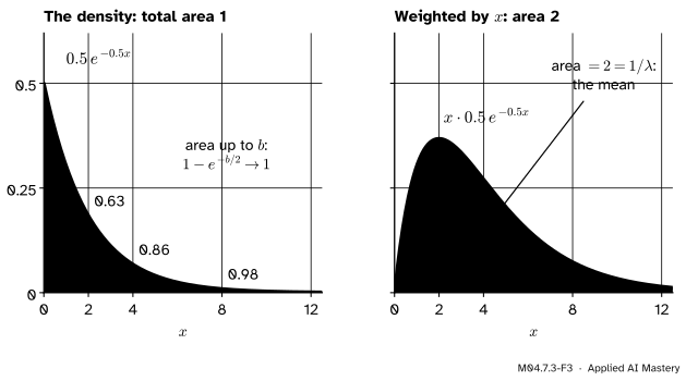
A waiting time. Suppose the time \(X\), in minutes, until the next request reaches a server has the density \({f(x) = \lambda e^{-\lambda x}}\) for \({x \ge 0}\) (and 0 for \({x < 0}\)), with \({\lambda = 0.5}\) per minute. This is an invented example, but the exponential density is a common model for waiting times. A density must be at least 0 everywhere and enclose a total area of 1, and the mean waiting time is the area under \({x\,f(x)}\).
Total area. An antiderivative of \({\lambda e^{-\lambda x}}\) is \({-e^{-\lambda x}}\) (differentiate to check). So
With \({\lambda = 0.5}\) the area up to \({b = 2, 4, 8}\) is 0.63, 0.86 and 0.98, closing in on 1.
The mean. Integrate \({x\,\lambda e^{-\lambda x}}\) by parts on \({[0, b]}\), with \({u = x}\) and \({dv = \lambda e^{-\lambda x}\,dx}\), so \({du = dx}\) and \({v = -e^{-\lambda x}}\):
As \(b\) grows, the last term tends to \({1/\lambda}\). The boundary term needs care: \({b\,e^{-\lambda b}}\) is a growing \(b\) times a shrinking \({e^{-\lambda b}}\). Which wins?
Why \({b\,e^{-b} \to 0}\): integrate \({e^t \ge 1}\) twice. For \({t \ge 0}\), \({e^t \ge 1}\). Integrating both sides from 0 to \(s\) keeps the inequality (a bigger function has a bigger integral, M04.5.3): \({e^s - 1 \ge s}\). Integrate again, from 0 to \(c\):
Hence \({0 < c\,e^{-c} = c/e^c < c \big/ \tfrac{c^2}{2} = 2/c}\), which tends to 0, and by the squeeze theorem (M04.1.2) \({c\,e^{-c} \to 0}\). With \({c = \lambda b}\), \({b\,e^{-\lambda b} = \frac{1}{\lambda}\,(\lambda b)\,e^{-\lambda b} \to 0}\). So the mean is
The exponential density with \({\lambda = 0.5}\). Left: the area up to \(b\) is 0.63, 0.86, 0.98 at \({b = 2, 4, 8}\), and tends to 1. Right: weighting by \(x\) gives a curve whose total area is the mean, \({1/\lambda = 2}\).
Code
From scratch, the areas up to \(b\) for growing \(b\), straight from the antiderivatives.
import math# Areas from the left end up to b: under 1/x^2, under 1/x, under the density 0.5 e^(-x/2),# and under x times that density (the mean up to b).print(f"{'b':>4}{'1/x^2':>6}{'1/x':>6}{'dens.':>6}{'mean':>6}")for b in (2, 4, 8, 10, 100, 1000): mean_b =-b * math.exp(-0.5* b) + (1- math.exp(-0.5* b)) /0.5print(f"{b:4d}{1-1/b:6.3f}{math.log(b):6.3f}{1- math.exp(-0.5* b):6.3f}{mean_b:6.3f}")
The column for \({1/x^2}\) settles on 1, the column for \({1/x}\) never settles, and the last two settle on 1 and on the mean, 2. The library takes infinite limits directly: pass numpy.inf to scipy.integrate.quad.
import numpy as npfrom scipy import integratechecks = [ ("1/x^2 on [1, inf)", lambda x: 1/ x**2, 1, np.inf, 1.0), ("1/sqrt(x) on (0, 1]", lambda x: 1/ np.sqrt(x), 0, 1, 2.0), ("0.5 e^(-x/2) on [0, inf)", lambda x: 0.5* np.exp(-0.5* x), 0, np.inf, 1.0), ("x 0.5 e^(-x/2) on [0, inf)", lambda x: x *0.5* np.exp(-0.5* x), 0, np.inf, 2.0), ("e^(-x^2/2) on the line", lambda x: np.exp(-x**2/2), -np.inf, np.inf, math.sqrt(2* math.pi)),]for name, f, a, b, exact in checks: value, error = integrate.quad(f, a, b)print(f"{name:27s}{value:.8f} exact {exact:.8f} error estimate {error:.0e}")
1/x^2 on [1, inf)           1.00000000   exact 1.00000000   error estimate 1e-14
1/sqrt(x) on (0, 1]         2.00000000   exact 2.00000000   error estimate 4e-15
0.5 e^(-x/2) on [0, inf)    1.00000000   exact 1.00000000   error estimate 4e-11
x 0.5 e^(-x/2) on [0, inf)  2.00000000   exact 2.00000000   error estimate 7e-10
e^(-x^2/2) on the line      2.50662827   exact 2.50662827   error estimate 3e-08
quad confirms the bell curve’s total area, \({\sqrt{2\pi}}\). That number is why the normal density carries the factor \({1/\sqrt{2\pi}}\): dividing by it makes the total area 1. But a number from quad is not a proof of convergence. Asked for the divergent \({\int_1^\infty dx/x}\), it still returns a finite number, with a warning.
import warningswith warnings.catch_warnings(record=True) as caught: warnings.simplefilter("always") value, error = integrate.quad(lambda x: 1/ x, 1, np.inf)print(f"quad says {value:.1f} (error estimate {error:.1f}), warnings: {[w.category.__name__for w in caught]}")
The warning is the only sign of trouble. The proof that \({\int_1^\infty dx/x}\) diverges is \({\ln b \to \infty}\), not anything a computer prints.
Explore
This module’s interactive, the substitution viewer, lives in lesson M04.7.1. It shows an improper integral in the making. Choose \({x\,e^{-x^2/2}}\) and drag \(b\) to the right: the area, \({1 - e^{-b^2/2}}\), creeps up towards 1, while the \(u\)-limit \({b^2/2}\) runs away. Let \(b\) go to infinity and the integral is \({\int_0^\infty x\,e^{-x^2/2}\,dx = 1}\).
Pitfalls
M04.7.3-F4
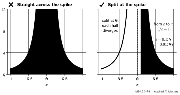
Wrong beside right for \({\int_{-1}^{1} dx/x^2}\). The fundamental theorem used straight across the spike gives \({-2}\), a negative area under a positive curve (left). Split at the spike: each half diverges (right).
“\({\int_{-1}^{1} dx/x^2}\) is \({\big[-1/x\big]_{-1}^{1}}\), which is \({-2}\).”
Part two of the fundamental theorem needs \(f\) continuous on the whole closed interval, and \({1/x^2}\) blows up at 0, inside it. Split there. On the right, \({\int_\varepsilon^1 dx/x^2 = 1/\varepsilon - 1}\), which is 9 at \({\varepsilon = 0.1}\) and 99 at \({0.01}\): it diverges, so the whole integral diverges. A negative answer for a positive integrand was the warning.
“The curve falls to zero, so the area must be finite.”
\({1/x}\) falls to zero and encloses infinite area. Falling to zero is not enough; falling fast enough is what counts, and \({1/x}\) is exactly the boundary: \({1/x^p}\) with \({p > 1}\) falls fast enough, and \({p \le 1}\) does not.
“\({\int_{-\infty}^{\infty} x\,dx = 0}\), by symmetry.”
The definition asks each half to converge on its own, and \({\int_0^b x\,dx = b^2/2}\) does not. The symmetric limit of \({\int_{-b}^{b} x\,dx}\) is 0, but that is a different, weaker quantity. The difference matters in practice: a density whose tails fall only like \({1/x^2}\) encloses a finite total area (\({p = 2}\)), but \({x}\) times it falls like \({1/x}\) (\({p = 1}\)), so it has no mean (exercise 2).
Frontier note: the normalising constant
Dividing \({e^{-x^2/2}}\) by \({\sqrt{2\pi}}\) makes it a density. Most models in machine learning are written the same way, as a positive function divided by its total area, called the normalising constant, an improper integral over all inputs. With many inputs that integral is usually out of reach: Hyvärinen (2005, Section 1) notes that for almost any dimension above 2, computing it numerically is practically impossible. Score matching (the box in lesson M04.7.2) and Monte Carlo methods (M07.10) exist to work around it.
Check yourself
Recall
1. How is \({\int_a^\infty f(x)\,dx}\) defined?
Show answer
As \({\lim_{b \to \infty} \int_a^b f(x)\,dx}\). It converges if that limit exists and is finite, and diverges otherwise.
2. For which \(p\) does \({\int_1^\infty dx/x^p}\) converge, and to what?
Show answer
Exactly for \({p > 1}\), and then it equals \({1/(p - 1)}\).
3. What is \({\int_0^1 dx/\sqrt{x}}\), and why is it improper?
Show answer
It is 2, the limit of \({2 - 2\sqrt{\varepsilon}}\). It is improper because \({1/\sqrt{x}}\) is unbounded near 0.
4. What two properties make \(f\) a probability density, and what is the mean of the density \({\lambda e^{-\lambda x}}\)?
Show answer
\({f \ge 0}\) everywhere and total area 1. The mean of the exponential density is \({1/\lambda}\).
5. Why is \({\int_{-1}^{1} dx/x^2}\) not \({-2}\)?
Show answer
The integrand blows up at 0, inside the interval, so the fundamental theorem does not apply. Split at 0: each half diverges, so the integral diverges.
Exercises
1.★ Find \({\int_1^\infty dx/x^3}\) and \({\int_0^\infty e^{-3x}\,dx}\).
Show solution
With \({p = 3}\), the result above gives \({1/(3 - 1) = 1/2}\). Directly: \({\int_1^b x^{-3}\,dx = \tfrac12 - \tfrac{1}{2b^2} \to \tfrac12}\). For the second, an antiderivative of \({e^{-3x}}\) is \({-\tfrac13 e^{-3x}}\), so \({\int_0^b e^{-3x}\,dx = \tfrac13 - \tfrac13 e^{-3b} \to \tfrac13}\).
2.★★ Show that \({\int_0^\infty \frac{x}{1 + x^2}\,dx}\) diverges.
which grows without bound. For large \(x\) the integrand is close to \({1/x}\), the boundary case \({p = 1}\). The density \({\frac{1}{\pi(1 + x^2)}}\), called the Cauchy density, has tails like \({1/x^2}\); this exercise shows that \({x}\) times it has no finite area, so it has no mean.
3.★★★ Use the antiderivative \({-(x^2 + 2x + 2)\,e^{-x}}\) from lesson M04.7.2 to show that \({\int_0^\infty x^2 e^{-x}\,dx = 2}\). You will need \({b^2 e^{-b} \to 0}\): prove it by integrating \({e^t \ge 1}\) three times.
Show solution
From 0 to \(b\), the integral is \({2 - (b^2 + 2b + 2)\,e^{-b}}\). Integrating \({e^t \ge 1}\) three times from 0 gives \({e^c \ge 1 + c + \frac{c^2}{2} + \frac{c^3}{6}}\), so \({e^c > c^3/6}\) for \({c > 0}\). Then
The worked example showed \({b\,e^{-b} \to 0}\), and \({2e^{-b} \to 0}\), so \({(b^2 + 2b + 2)\,e^{-b} \to 0}\) and the integral is 2. The same steps give \({\int_0^\infty x^n e^{-x}\,dx = n!}\): the constant left at \({x = 0}\) by the antiderivative is \({n!}\), and every other term vanishes at both ends.
Summary card
An area out to infinity is the limit of the areas up to \(b\): it may settle, or it may not.
M04.7.3-F1
\({1/x^2}\) settles at 1; \({1/x}\) never settles.
Definition.\({\int_a^\infty f = \lim_{b \to \infty}\int_a^b f}\); a spike: \({\lim_{\varepsilon \to 0^+}}\).
The \({p}\) rule.\({\int_1^\infty x^{-p}\,dx = \frac{1}{p - 1}}\) for \({p > 1}\), divergent for \({p \le 1}\).
Sources. Each was opened and checked against this lesson on 12 November 2026.
Gilbert Strang and Edwin Herman, Calculus Volume 2 (OpenStax), Section 3.7, Improper integrals: the definitions for infinite ranges (Equations 3.16 to 3.18, with both halves required to converge on the whole line) and for discontinuous integrands (Equations 3.19 to 3.21), Example 3.47 (the infinite area under \({1/x}\)), Theorem 3.7 (a comparison theorem) and Example 3.49, an exponential density.
Matthew Boelkins, Active Calculus (single variable), Section 6.5, Improper integrals: \({\int_0^1 dx/\sqrt{x} = 2}\) found as a limit (Subsection 6.5.4), and the summary (Subsection 6.5.5) that \({\int_1^\infty dx/x^p}\) converges for \({p > 1}\) and diverges for \({0 < p \le 1}\).
David Jerison, MIT OpenCourseWare 18.01SC, Session 91, Improper integrals: the notes of the clip Introduction to improper integrals define the improper integral as the limit of the integrals from \(a\) to \(N\), converging when that limit exists, with the picture of an area that stretches to infinity; a later clip of the session treats \({1/x^p}\).
Aapo Hyvärinen, Estimation of non-normalized statistical models by score matching, Journal of Machine Learning Research 6 (2005), Section 1: the normalising constant as an integral that is often intractable, and practically impossible to compute numerically in more than two dimensions.
Next.M04.7.4 Simpson’s rule and quad computes areas under the bell curve, which has no antiderivative to write down, and so finds the normal probabilities.