The lowest point of a bowl: the least-squares line
At the lowest point of a smooth surface both partial derivatives are zero. Set them to zero for the mean squared error of a line through four points, solve the two equations, and prove the answer is the lowest point: the least-squares line y-hat = 1.4x + 0.5.
Explain, from Fermat’s theorem applied to each slice, why both partial derivatives are zero at an interior lowest point.
Derive the two partial derivatives of the mean squared error of a line with the chain rule.
Solve the two resulting equations by substitution to find the least-squares line of a small dataset.
Show that a flat point need not be a lowest point, and prove that the answer here is the lowest by writing the loss as two squares plus a constant.
Check the answer with central differences, scipy.optimize.minimize and numpy.polyfit.
In review. The maths and code on this page are checked by automated tests on every change, but an independent reader has not signed it off yet. Spot a mistake or a confusing step? Tell us.
The question
Four points, one best line: which slope \(w\) and intercept \(b\) make the mean squared error as small as it can be? With one parameter you set the derivative to zero (M04.4). With two, what are the equations, and how can you be sure the answer is the lowest point and not just a flat one? The answer, the least-squares line, is one of the few training results with an exact formula, so it is the yardstick that step-by-step training methods are checked against.
From the last lesson
1. In which direction is the slope of \(f\) largest, and how large is it?
Show answer
Along the gradient, and the slope there is the gradient’s length. For the running bowl at \({(1, 1)}\) that is \({(2, 4)}\), of length \({\sqrt{20} \approx 4.47}\).
2. Which directions have slope zero, and what are they on the map?
Show answer
The two at right angles to the gradient: the directions of the contour line through the point.
Intuition
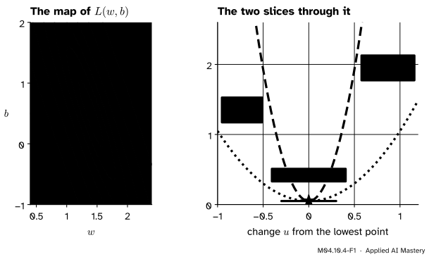
Stand at the bottom of a bowl and look along any slice through your feet. Every slice is at its own bottom there, or the bowl would go lower. In particular the slice along \(w\) is at its bottom, so its slope is zero, and so is the slope of the slice along \(b\).
M04.10.4-F1
The two slices through the lowest point of the loss. Each is at its own bottom there, so both are flat: both partial derivatives are zero.
So at the lowest point \({\pd{L}{w} = 0}\) and \({\pd{L}{b} = 0}\): two equations for the two unknowns \(w\) and \(b\). Solve them and you have the candidate. Then one more question remains, because a surface can be flat in both directions without being at its bottom.
Build it up
Step 1. One slice, one equation. Suppose the lowest point is \({(w^*, b^*)}\). Freeze \({b = b^*}\). The slice \({L(w, b^*)}\) is an ordinary function of \(w\), and its lowest value is at \({w = w^*}\), because no point of the surface is lower. By Fermat’s theorem (M04.4.1) its slope is zero there, and that slope is \({\pd{L}{w}}\).
Step 2. The other slice, the other equation. Freeze \({w = w^*}\) instead. The same argument gives \({\pd{L}{b} = 0}\).
Step 3. Solve. Two equations in two unknowns usually pin down one point: the candidate.
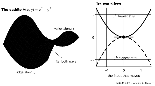
Step 4. Flat is not enough. The saddle \({h(x, y) = x^2 - y^2}\) has \({\pd{h}{x} = 2x}\) and \({\pd{h}{y} = -2y}\), both zero at the origin. Yet along \(x\) the origin is the bottom of a valley, \({h(x, 0) = x^2}\), and along \(y\) the top of a ridge, \({h(0, y) = -y^2}\). It is neither a lowest nor a highest point.
M04.10.4-F2
The saddle \({x^2 - y^2}\). At the middle both slopes are zero, but one slice has its lowest point there and the other its highest.
The formal statement
NoteTheorem: Fermat’s theorem for two inputs
If \(f\) has a local minimum or a local maximum at a point \({(a, b)}\) that is not on the edge of its domain, and both partial derivatives exist there, then
\[
\pd{f}{x}(a, b) = 0 \quad\text{and}\quad \pd{f}{y}(a, b) = 0 .
\]
Proof. Take a local minimum. Near \({(a, b)}\) no value of \(f\) is lower than \({f(a, b)}\). The slice \({g(x) = f(x, b)}\) looks only at points near \({(a, b)}\) when \(x\) is near \(a\), so \({g(x) \geq g(a)}\) there: \(g\) has a local minimum at \(a\), an inner point of its domain. By Fermat’s theorem in one variable, \({g'(a) = 0}\). But \({g'(a)}\) is, by definition, \({\pd{f}{x}(a, b)}\). The slice \({y \mapsto f(a, y)}\) gives \({\pd{f}{y}(a, b) = 0}\) in the same way, and a maximum works alike.
A point where both partial derivatives are zero, or where one of them does not exist, is a critical point. A critical point that is neither a local minimum nor a local maximum, like the middle of the saddle, is a saddle point.
The slopes of the loss. The loss is the mean of the squared residuals,
\[
L(w, b) = \frac{1}{n} \sum_{i=1}^{n} (w x_i + b - y_i)^2 ,
\]
with \({n = 4}\). A constant factor and a sum pass through the derivative, and lesson 2 found the slope of each squared term with the chain rule. So
\[
\begin{aligned}
\pd{L}{w} &= \frac{2}{n} \sum_{i=1}^{n} (w x_i + b - y_i)\, x_i , \\
\pd{L}{b} &= \frac{2}{n} \sum_{i=1}^{n} (w x_i + b - y_i) .
\end{aligned}
\]
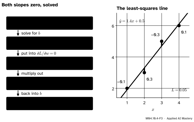
Multiply each bracket out and add over the points, using \({\sum x_i = 10}\), \({\sum x_i^2 = 30}\), \({\sum x_i y_i = 47}\) and \({\sum y_i = 16}\), and \(b\) added once per point:
so \({w = 1.4}\), and then \({b = 4 - 2.5 \times 1.4 = 4 - 3.5 = 0.5}\). The candidate is the line \({\hat{y} = 1.4x + 0.5}\). Its predictions are 1.9, 3.3, 4.7 and 6.1, its residuals \({-0.1, 0.3, -0.3, 0.1}\), and its loss is \({(0.01 + 0.09 + 0.09 + 0.01)/4 = 0.05}\).
M04.10.4-F3
The worked example as a trace. Substitution turns the two equations into one, then back into the other; the line it gives misses each point by at most 0.3.
Is it the lowest point? Being flat is not enough, as the saddle showed, so write the loss in a form that shows its lowest value. Start from the multiplied-out loss of lesson 1 and collect the terms with \(b\):
Complete the square in \(b\) (M01.3.3): \({b^2 + (5w - 8)b} = {(b + 2.5w - 4)^2 - (2.5w - 4)^2}\), and \({(2.5w - 4)^2 = 6.25w^2 - 20w + 16}\). So
\[
\begin{aligned}
L &= (2.5w + b - 4)^2 \\
&\quad + 1.25w^2 - 3.5w + 2.5 .
\end{aligned}
\]
Complete the square in \(w\) too: \({1.25w^2 - 3.5w} = {1.25(w - 1.4)^2 - 2.45}\). Altogether
\[
\begin{aligned}
L &= (2.5w + b - 4)^2 \\
&\quad + 1.25\,(w - 1.4)^2 + 0.05 .
\end{aligned}
\]
Squares are never negative, so \({L \geq 0.05}\) for every line, and \({L = 0.05}\) only when both squares are zero: \({w = 1.4}\) and then \({b = 4 - 3.5 = 0.5}\). So \({(1.4, 0.5)}\) is the lowest point of the whole surface, not merely a flat one, and no other line does as well.
Code
First from scratch: the sums, the two equations solved by substitution, and both slopes checked by central differences at the answer.
x = [1.0, 2.0, 3.0, 4.0]y = [2.0, 3.0, 5.0, 6.0]n =len(x)sx, sxx =sum(x), sum(v * v for v in x)sy, sxy =sum(y), sum(a * b for a, b inzip(x, y))# The two slopes as numbers: dL/dw = a1 w + c1 b - e1 and dL/db = a2 w + c2 b - e2.a1, c1, e1 =2* sxx / n, 2* sx / n, 2* sxy / na2, c2, e2 =2* sx / n, 2.0, 2* sy / nprint(f"dL/dw = {a1} w + {c1} b - {e1}")print(f"dL/db = {a2} w + {c2} b - {e2}")# Substitution, as in the worked example: dL/db = 0 gives b = (e2 - a2 w) / c2.w = (e1 - c1 * e2 / c2) / (a1 - c1 * a2 / c2)b = (e2 - a2 * w) / c2def loss(w, b):returnsum((w * xi + b - yi) **2for xi, yi inzip(x, y)) / nh =1e-5dw = (loss(w + h, b) - loss(w - h, b)) / (2* h)db = (loss(w, b + h) - loss(w, b - h)) / (2* h)print(f"w = {w:.4f}, b = {b:.4f}, L = {loss(w, b):.4f}")print(f"slopes there: {dw:.1e} and {db:.1e}")
dL/dw = 15.0 w + 5.0 b - 23.5
dL/db = 5.0 w + 2.0 b - 8.0
w = 1.4000, b = 0.5000, L = 0.0500
slopes there: 0.0e+00 and 4.2e-12
The slopes at the answer are zero up to rounding. Now two library routes. scipy.optimize.minimize searches for the lowest point of any function from a starting guess; with no bounds or constraints it uses the BFGS method, which follows slopes it estimates as it goes. numpy.polyfit(x, y, 1) fits the least-squares line directly and returns its coefficients, highest power first.
The search only gets close, to four decimals here, and its last digits can differ from one computer to another. The two equations give the answer exactly.
Explore
This module’s interactive, the slope compass, lives in lesson M04.10.3. Choose the loss and press To the flat point: the point jumps to \({(1.4, 0.5)}\), both slopes read 0 and the dial is flat in every direction. Then choose the saddle and do the same: flat again, but the side panels show one valley and one ridge.
Pitfalls
M04.10.4-F4
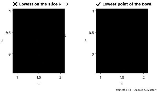
Wrong beside right. The best slope with the intercept held at 0 is flat along \(w\) only; the way down still leads up in \(b\), to the star.
“Tune each parameter to its best value and you are at the bottom.”
The running loss of this course is the slice \({b = 0}\), and its lowest point is \({w = 47/30}\), where \({L \approx 0.092}\). There \({\pd{L}{w} = 0}\), but \({\pd{L}{b}} = {5 \times 47/30 - 8} = {-1/6}\): raising \(b\) still lowers the loss, down to 0.05 at the star. One parameter at a time finds the bottom of a slice. Both slopes must be zero at once.
“Both partial derivatives are zero, so it is a minimum.”
The middle of the saddle \({x^2 - y^2}\) is flat both ways and is neither. Zero slopes make a point a candidate. Here the two-squares form proved the candidate is the lowest point; course M05 gives the general test with second derivatives.
“Setting one partial derivative to zero finds the point.”
One equation in two unknowns leaves a whole line of solutions: every point of \({5w + 2b = 8}\) is the bottom of its own \(b\)-slice. Only both equations together fix one point.
Check yourself
Recall
1. Why are both partial derivatives zero at an interior lowest point?
Show answer
Each slice through the point has its own lowest point there, so by Fermat’s theorem each slice’s slope, which is a partial derivative, is zero.
2. What is a critical point, and what is a saddle point?
Show answer
A critical point has both partial derivatives zero, or one of them missing. A saddle point is a critical point that is neither a local minimum nor a local maximum.
3. What are the two partial derivatives of the loss of the four points?
4. What is the least-squares line for the four points, and its loss?
Show answer
\({\hat{y} = 1.4x + 0.5}\), with \({L = 0.05}\).
5. How does the two-squares form prove that \({(1.4, 0.5)}\) is the lowest point?
Show answer
\({L} = {(2.5w + b - 4)^2} + {1.25(w - 1.4)^2} + {0.05}\). Squares are never negative, so \({L \geq 0.05}\), with equality only when both squares are zero, at \({(1.4, 0.5)}\).
Exercises
1.★ Find the critical point of \({f(x, y) = x^2 + 2y^2 - 4x + 4y}\), and show by completing squares that it is the lowest point.
with equality only at \({(2, -1)}\): the running bowl moved to a new centre and lowered by 6.
2.★★ Fit the line \({\hat{y} = wx + b}\) to the three points \({(0, 1)}\), \({(1, 3)}\) and \({(2, 2)}\) by setting both partial derivatives of the mean squared error to zero.
Show solution
Here \({n = 3}\), \({\sum x_i = 3}\), \({\sum x_i^2 = 5}\), \({\sum y_i = 6}\) and \({\sum x_i y_i = 0 + 3 + 4 = 7}\). So \({\pd{L}{w} = \tfrac23(5w + 3b - 7)}\) and \({\pd{L}{b} = \tfrac23(3w + 3b - 6)}\). Setting both to zero: \({5w + 3b = 7}\) and \({3w + 3b = 6}\). Subtracting the second from the first gives \({2w = 1}\), so \({w = 0.5}\), and then \({3b = 6 - 1.5}\), so \({b = 1.5}\). The line is \({\hat{y} = 0.5x + 1.5}\). Its residuals are 0.5, \(-1\) and 0.5, and \({L = (0.25 + 1 + 0.25)/3 = 0.5}\).
3.★★★ Let \({g(w, b) = w^2 + 4wb + b^2}\). (a) Show that \({(0, 0)}\) is its only critical point. (b) Show that it is a saddle point. (c) Why does completing squares not prove a minimum here, when it did for the loss?
Show solution
(a) \({\pd{g}{w} = 2w + 4b}\) and \({\pd{g}{b} = 4w + 2b}\). The first is zero when \({w = -2b}\); then the second is \({-8b + 2b = -6b}\), zero only at \({b = 0}\), so \({w = 0}\) too.
(b) Along \({b = 0}\), \({g(t, 0) = t^2 > 0}\) for \({t \neq 0}\). Along \({b = -w}\), \({g(t, -t)} = {t^2 - 4t^2 + t^2} = {-2t^2 < 0}\). Arbitrarily close to the origin there are higher and lower values, so it is neither a minimum nor a maximum.
(c) Completing the square gives \({g = (w + 2b)^2 - 3b^2}\). The second square comes with a minus sign, so \(g\) falls along the directions where \({w + 2b = 0}\). For the loss both squares had plus signs.
Summary card
At the lowest point of a smooth surface both slopes are zero; for a line’s squared error, solving those two equations gives the best line.
M04.10.4-F1
Both slices flat at the bottom.
Fermat, once per input: at an inner lowest point, \({\pd{f}{x} = 0}\) and \({\pd{f}{y} = 0}\).
Flat is not lowest: \({x^2 - y^2}\) has a saddle point at the origin.
Both zero at \({w = 1.4}\), \({b = 0.5}\): the line \({\hat{y} = 1.4x + 0.5}\), \({L = 0.05}\).
Two squares prove it is the lowest: \({L} = {(2.5w + b - 4)^2} + {1.25(w - 1.4)^2} + {0.05}\).
Sources and next steps
Sources. Each was opened and checked against this lesson on 12 November 2026.
Gilbert Strang and Edwin Herman, Calculus Volume 3 (OpenStax), Section 4.7: the definition of a critical point (both partial derivatives zero, or one of them missing), Theorem 4.16 (Fermat’s theorem for functions of two variables), and the definition of a saddle point, with the surface \({x^2 - y^2}\) and its downward trace \({z = -y^2}\).
SciPy 1.18 reference, scipy.optimize.minimize: the method is chosen by whether the problem has bounds or constraints, the default for an unconstrained problem is BFGS, and the result’s x holds the solution.
NumPy 2.5 reference, numpy.polyfit: a least squares polynomial fit that minimises the sum of squared errors and returns the coefficients highest power first.