A map with several inputs and several outputs bends the grid, but close to any point it acts like a matrix. Meet the Jacobian: its rows are the gradients of the outputs, its columns say where a small step along each input goes.
M05.4.1L2 Intermediate25 minIn review (what this means)
The maths and code on this page are checked by automated tests on every change, but an independent reader has not signed it off yet. Spot a mistake or a confusing step? Tell us.
Define the Jacobian of a map from R^n to R^m through its linear approximation, and state its shape.
Compute a Jacobian entry by entry from partial derivatives, and read it by rows (gradients) and by columns (images of small steps).
Work out the Jacobians of the linear map T, the polar map and the running warp at given points, and check a prediction against the true change.
Build a Jacobian from central differences and compare it with scipy.differentiate.jacobian, paying attention to the output shape.
The question
A gradient tells you how one output responds to a small nudge of all the inputs. But a layer of a network, an image warp or a change of coordinates has many outputs. Nudge the inputs a little: how does every output move, and is there one object that holds the whole answer?
Intuition
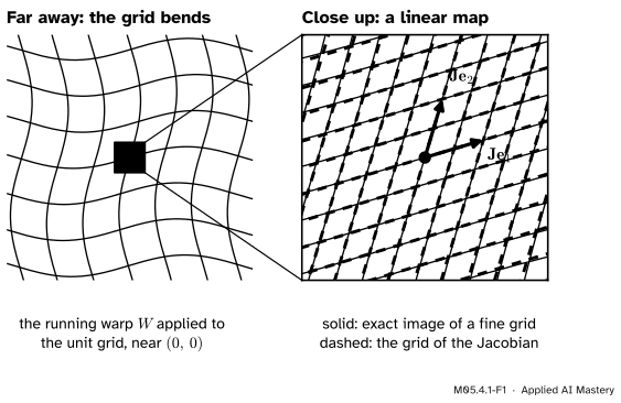
Take a smooth map of the plane and draw what it does to a grid. Far away the grid lines bend. Now zoom in on one point. The closer you look, the straighter the lines become, until the grid near the point looks like a grid of identical parallelograms: the picture of a linear map (M02.4).
M05.4.1-F1
The running warp \({W(x, y) = (x + 0.3\sin y,\; y + 0.3\sin x)}\). Far away it bends the grid. Close to the origin its image is the grid of a single matrix, the Jacobian, whose two columns are the arrows.
That matrix is the Jacobian. It is to a map with many outputs what the slope is to a function of one variable and the gradient is to a function of many: the best linear stand-in near one point. And it is still a matrix, so everything from linear algebra applies to it, one point at a time.
Build it up
Step 1. A map is a stack of functions. A map \(f\) from \(\R^n\) to \(\R^m\) takes \(n\) inputs and gives \(m\) outputs, so it is \(m\) ordinary functions written one above another: \({f(\vect{x})} = {(f_1(\vect{x}), \dots, f_m(\vect{x}))}\). The running warp has two: \({f_1 = x + 0.3\sin y}\) and \({f_2 = y + 0.3\sin x}\).
Step 2. Linearise each one. Each \(f_i\) is a function with one output, so lesson M05.2.2 gives its linear approximation near a point \(\vect{a}\), for a small step \(\vect{h}\):
Step 3. Stack the \(m\) approximations. Write the \(m\) row vectors \({\nabla f_i(\vect{a})\T}\) one under another. They make an \(m \times n\) matrix \(\mat{J}\), and the \(m\) approximations become one:
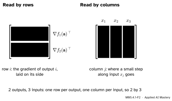
Step 4. Read the matrix two ways. Row \(i\) is the gradient of output \(i\), laid on its side. Column \(j\) is \({\mat{J}\vect{e}_j}\), the predicted change when the step is one unit along input \(j\) alone. So column \(j\) says where a small step along input \(x_j\) goes.
M05.4.1-F2
The same Jacobian read two ways: by rows, one gradient per output; by columns, one small step per input.
The formal statement
NoteDefinition: differentiable map and Jacobian
A map \(f\) from \(\R^n\) to \(\R^m\) is differentiable at \(\vect{a}\) if there is an \(m \times n\) matrix \(\mat{J}\) such that, for every small step \(\vect{h}\),
where the remainder \(r(\vect{h})\), a vector in \(\R^m\), satisfies \({\norm{r(\vect{h})} / \norm{\vect{h}} \to 0}\) as \({\vect{h} \to \vect{0}}\). The matrix is the Jacobian of \(f\) at \(\vect{a}\), written \({\mat{J}_f(\vect{a})}\).
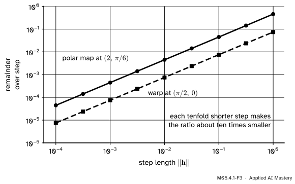
The condition says the error is small even compared with the step. Any matrix makes the error small when \(\vect{h}\) is small; only one makes it small faster than \(\vect{h}\), and that is why the Jacobian is the best linear approximation.
M05.4.1-F3
The definition, measured. For both maps the remainder divided by the step length falls tenfold for each tenfold shorter step: it tends to 0, as the definition asks.
The entries are partial derivatives. Take the step along one input axis, \({\vect{h} = s\,\vect{e}_j}\) with a small number \(s\). Then \({\mat{J}\vect{h} = s\,\mat{J}\vect{e}_j}\) and the definition reads
As \({s \to 0}\) the last term tends to \(\vect{0}\), because its length is \({\norm{r(s\vect{e}_j)} / \norm{s\vect{e}_j}}\). So the left side tends to \({\mat{J}\vect{e}_j}\), the \(j\)-th column. But entry \(i\) of the left side is the difference quotient of \(f_i\) in input \(x_j\), whose limit is the partial derivative \({\pd{f_i}{x_j}}\). Hence
Shape. One row per output, one column per input: \(m \times n\). This is the numerator layout that the course uses throughout.
One output. For \({m = 1}\) the Jacobian is the single row \({\nabla f(\vect{a})\T}\). The gradient is a column with the shape of the input, and the Jacobian is that column laid on its side.
Linear maps. For \({f(\vect{x}) = \mat{A}\vect{x}}\), \({f(\vect{a} + \vect{h}) = \mat{A}\vect{a} + \mat{A}\vect{h}}\) exactly, with no remainder, so \({\mat{J} = \mat{A}}\) at every point: a linear map is its own Jacobian.
Go deeper: when does the Jacobian exist?
The length of a vector tends to 0 exactly when each of its entries does, so \(f\) is differentiable exactly when every component \(f_i\) is. Lesson M05.2.2 showed that a function whose partial derivatives exist near \(\vect{a}\) and are continuous at \(\vect{a}\) is differentiable there (Theorem 4.7 of OpenStax Calculus Volume 3). So if all \({mn}\) partial derivatives are continuous, the Jacobian exists. Every map in this module is built from polynomials, sines and cosines, so its partial derivatives are continuous everywhere. Partial derivatives on their own are not enough; the pitfalls below show why.
Worked example
The linear map \({T(x, y) = (x + y,\; -x + 2y)}\). The partial derivatives of \({x + y}\) are 1 and 1; those of \({-x + 2y}\) are \(-1\) and 2. So
at every point: the matrix of \(T\) itself, as the formal statement predicts.
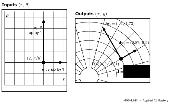
The polar map \({P(r, \theta) = (r\cos\theta,\; r\sin\theta)}\) at \({(2, \pi/6)}\). Differentiate each output in each input, the other input held fixed:
Read the columns. Column 1, \({(0.866, 0.5)}\), has length 1 and points straight out from the centre: raising \(r\) by a little moves the point outwards by the same amount. Column 2, \({(-1, 1.732)}\), has length 2 and points round the circle: turning \(\theta\) by a small angle sweeps an arc \(r\) times as long.
M05.4.1-F4
The polar map at \({(2, \pi/6)}\). A unit step in \(r\) goes to the first column, a unit step outwards; a unit step in \(\theta\) goes to the second, a step of length 2 round the circle.
Check a prediction. Step \({\vect{h} = (0.1, 0.05)}\). The Jacobian predicts the output moves by \({\mat{J}\vect{h}} \approx {(0.0866 - 0.05,\; 0.05 + 0.0866)} = {(0.037, 0.137)}\). The true move, \({P(2.1, \pi/6 + 0.05) - P(2, \pi/6)}\), is about \({(0.032, 0.140)}\). The remainder has length about 0.0056, which is 5% of the step’s length 0.112; halve the step and the share halves too.
The running warp \(W\). Its outputs are \({x + 0.3\sin y}\) and \({y + 0.3\sin x}\), and their partial derivatives give
\[
\mat{J}_W = \begin{bmatrix} 1 & 0.3\cos y \\ 0.3\cos x & 1 \end{bmatrix} .
\]
At \({(0, 0)}\) both cosines are 1, so \({\mat{J}_W = \begin{bmatrix} 1 & 0.3 \\ 0.3 & 1 \end{bmatrix}}\): a step along \(x\) also lifts \(y\) by 0.3 of the step, and a step along \(y\) pushes \(x\) the same way. That is the slant of the parallelograms in the anchor picture. At \({(\pi/2, 0)}\), \({\cos(\pi/2) = 0}\), so \({\mat{J}_W = \begin{bmatrix} 1 & 0.3 \\ 0 & 1 \end{bmatrix}}\), a shear. The same map has a different Jacobian at every point. A step of \({(0.1, 0.1)}\) from \({(\pi/2, 0)}\) is predicted to move the output by \({(0.13, 0.1)}\); the true move is about \({(0.12995, 0.09850)}\).
Code
From scratch: column \(j\) of the Jacobian is a central difference along input \(j\), so the whole matrix costs \({2n}\) evaluations of \(f\).
import numpy as npdef jacobian_fd(f, a, h=1e-6):"""Jacobian of f at a by central differences, one column per input.""" a = np.asarray(a, dtype=float) columns = []for j inrange(a.size): e = np.zeros_like(a) e[j] = h columns.append((np.asarray(f(a + e)) - np.asarray(f(a - e))) / (2* h))return np.column_stack(columns)def polar(v): r, th = vreturn np.array([r * np.cos(th), r * np.sin(th)])def warp(v): x, y = vreturn np.array([x +0.3* np.sin(y), y +0.3* np.sin(x)])def g(v): # three inputs, two outputs x1, x2, x3 = vreturn np.array([x1 * x2, x2 + x3 **2])a = np.array([2.0, np.pi /6])print("polar at (2, pi/6):\n", jacobian_fd(polar, a).round(4))print("warp at (pi/2, 0):\n", jacobian_fd(warp, [np.pi /2, 0]).round(4))print("g at (1, 2, 3), shape", jacobian_fd(g, [1, 2, 3]).shape, "\n", jacobian_fd(g, [1, 2, 3]).round(4))h = np.array([0.1, 0.05])true_move = polar(a + h) - polar(a)predicted = jacobian_fd(polar, a) @ hprint("true move", true_move.round(4), " predicted", predicted.round(4)," remainder / step", round(np.linalg.norm(true_move - predicted) / np.linalg.norm(h), 4))
SciPy’s scipy.differentiate.jacobian does the same job with a higher-order difference formula and an error estimate. Its function must accept a whole batch of points, with the inputs along the first axis, which our three maps already do. Its documentation calls the number of inputs \(m\) and of outputs \(n\), the other way round from this course; in our letters, the result df has shape \(m \times n\), one row per output.
Pick a map and drag the orange point, or set it with the sliders. The black outline is the exact image of a small square with a corner at the point; the dashed shape is the parallelogram the Jacobian predicts. Press Shrink the square and watch the close-up: the two become one shape. For the linear map they agree at every size.
Pitfalls
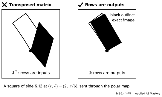
M05.4.1-F5
Wrong beside right. The transposed matrix predicts a parallelogram leaning the wrong way; the Jacobian, one row per output, matches the exact image.
“Each row of the Jacobian belongs to one input.”
Each row belongs to one output, each column to one input. Swap them and the prediction \({\mat{J}\T\vect{h}}\) is wrong whenever \(\mat{J}\) is not symmetric, as the picture shows, and for a map from \(\R^3\) to \(\R^2\) the product does not even have the right size. Some books use the transposed layout; check before you copy a formula.
“For a function with one output, the Jacobian is the gradient.”
It is the gradient laid on its side: a \(1 \times n\) row, \({\mat{J} = \nabla f\T}\). In this course the gradient is a column with the shape of the input, so that a step \({\vect{w} - \eta\nabla L}\) makes sense. Mathematics for Machine Learning writes the gradient as the row itself; the numbers are the same, the shape is not.
“All the partial derivatives exist, so the Jacobian is the best linear approximation.”
Take \({f(x, y) = xy/(x^2 + y^2)}\) with \({f(0, 0) = 0}\) (M05.1.4). Along each axis \(f\) is 0, so both partial derivatives at the origin are 0 and the only candidate is the row \({[\,0\;\;0\,]}\). But on the diagonal \({f(t, t) = 1/2}\) for every \({t \neq 0}\), so the remainder stays at \(1/2\) while the step shrinks: the ratio blows up. The function is not differentiable there, and no matrix describes it.
“The Jacobian describes the whole map.”
It describes the map near one point. The running warp has \({\begin{bmatrix} 1 & 0.3 \\ 0.3 & 1 \end{bmatrix}}\) at the origin and a shear at \({(\pi/2, 0)}\). Far from the point, the linear prediction drifts away from the truth, which is exactly what the remainder measures.
Check yourself
Recall
1. What shape is the Jacobian of a map from \(\R^n\) to \(\R^m\), and what is its entry \((i, j)\)?
Show answer
\(m \times n\), one row per output and one column per input. Entry \((i, j)\) is \({\pd{f_i}{x_j}}\).
2. What does column \(j\) of the Jacobian tell you?
Show answer
Where a small step along input \(x_j\) goes: a step of \(s\) along \(x_j\) moves the output by about \(s\) times column \(j\).
3. What makes \(\mat{J}\) the best linear approximation?
Show answer
The remainder \({f(\vect{a} + \vect{h}) - f(\vect{a}) - \mat{J}\vect{h}}\) shrinks faster than the step: its length divided by \({\norm{\vect{h}}}\) tends to 0. Only one matrix can do that.
4. What is the Jacobian of \({f(\vect{x}) = \mat{A}\vect{x}}\)?
Show answer
\(\mat{A}\), at every point. A linear map is its own Jacobian.
5. What are the Jacobian’s two columns for the polar map at \({(r, \theta)}\), and what do they look like?
Show answer
\({(\cos\theta, \sin\theta)}\), a unit step straight outwards, and \({(-r\sin\theta, r\cos\theta)}\), a step of length \(r\) round the circle.
Exercises
1.★ Find the Jacobian of \({f(x, y) = (x^2 y,\; x + \sin y)}\) at \({(1, 0)}\).
Show solution
The partial derivatives are \({\pd{}{x}(x^2y) = 2xy}\), \({\pd{}{y}(x^2y) = x^2}\), \({\pd{}{x}(x + \sin y) = 1}\) and \({\pd{}{y}(x + \sin y) = \cos y}\). At \({(1, 0)}\):
2.★★ The running loss of M04.10 fits \({\hat{y} = wx + b}\) to the inputs \({x = 1, 2, 3, 4}\). Write the four predictions as a map from \({(w, b)}\) to \(\R^4\). What is its Jacobian, and how much do the predictions move if \(w\) grows by 0.1?
Show solution
The map sends \({(w, b)}\) to the four predictions
\[
(w + b,\; 2w + b,\; 3w + b,\; 4w + b) .
\]
Each prediction has partial derivative \(x_i\) in \(w\) and 1 in \(b\), so
a \(4 \times 2\) matrix: the design matrix \(\mat{X}\) of the course, constant because the map is linear. A step of 0.1 in \(w\) moves the predictions by 0.1 times column 1: \({(0.1, 0.2, 0.3, 0.4)}\).
3.★★★ Show that the two columns of the polar Jacobian are perpendicular at every point, with lengths 1 and \(r\). What does this say about the image of a small square \({[r, r + s] \times [\theta, \theta + s]}\)?
Show solution
The dot product of the columns is \({\cos\theta\,(-r\sin\theta) + \sin\theta\,(r\cos\theta) = 0}\), so they are perpendicular. Their lengths are \({\sqrt{\cos^2\theta + \sin^2\theta} = 1}\) and \({\sqrt{r^2\sin^2\theta + r^2\cos^2\theta} = r}\). The image of the square is close to the parallelogram spanned by \(s\) times the columns: a rectangle with sides \(s\) and \({rs}\), so its area is about \({r s^2}\), \(r\) times the area of the square. Lesson M05.4.4 turns this into the Jacobian determinant.
Summary card
Close to a point, a smooth map is a matrix: the Jacobian.
Sources. Each was opened and checked against this lesson on 15 November 2026.
Gilbert Strang and Edwin Herman, Calculus Volume 3 (OpenStax), Section 4.4: differentiability with an error term that vanishes faster than the distance (Equation 4.26), and Theorem 4.7, continuous partial derivatives imply differentiability.
Marc Peter Deisenroth, A. Aldo Faisal and Cheng Soon Ong, Mathematics for Machine Learning, Section 5.3: Definition 5.6, the Jacobian as the \(m \times n\) matrix of partial derivatives (Equation 5.58), and the remark on the numerator layout used here. The book writes the gradient of a scalar function as a row.
Paige Bright, Alan Edelman and Steven G. Johnson, Matrix Calculus (for Machine Learning and Beyond), notes for MIT 18.S096, Section 2.4: the Jacobian as the \(m \times n\) linear operator with \({df = \mat{J}\,dx}\), and Example 11, the map \({\mat{A}\vect{x}}\) is its own Jacobian.
SciPy 1.18 reference, scipy.differentiate.jacobian: the function must accept inputs along the first axis; central differences by default; the attribute df has one row per output and one column per input.