Two more anomaly scores, the PCA reconstruction error and the one-class SVM, then a fair contest: every detector of the module on load_breast_cancer with ten planted malignant rows, judged by precision at k and average precision, and why ROC AUC flatters a detector when anomalies are rare.
ML03.9.4L2 Intermediate30 minIn review (what this means)
The maths and code on this page are checked by automated tests on every change, but an independent reader has not signed it off yet. Spot a mistake or a confusing step? Tell us.
Use the PCA reconstruction error as an anomaly score, and say which anomalies it can and cannot see.
Describe the one-class SVM from its picture in feature space, and state what nu bounds.
Compute precision at k, average precision and ROC AUC by hand for a ranked list.
Explain why ROC AUC flatters a detector when anomalies are rare, using the expected number of normal points ranked above an anomaly.
Compare the detectors of the module on load_breast_cancer with planted anomalies, using the labels only to judge.
The question
You now have four kinds of score, and on real data they disagree. A clinic has 367 biopsy records, of which 10 later proved malignant. Before trusting a detector with tomorrow’s records you want to know which one would have put those 10 at the top of the list. With anomalies under 3 % of the data, which number tells you that honestly?
From the last lesson
1. What anomaly score does a point get when its average path length equals \(c(n)\)?
Show answer
\({s = 2^{-c(n)/c(n)} = 2^{-1} = 0.5}\): a typical point.
2. Why does an isolation forest grow each tree on a small subsample?
Show answer
Small samples thin out clumps of anomalies and the normal points crowding them, which reduces masking and swamping; they also make the forest fast. The default is 256 points per tree.
Intuition
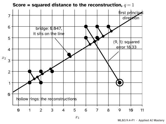
Normal data often lie close to a flat sheet, a low-dimensional subspace, even when they have many features. Compress every point onto that sheet and back, and normal points come back almost unchanged. A point that breaks the pattern comes back far from where it started.
ML03.9.4-F1
PCA with one component on the twelve points. The reconstruction error is the length of each reddish purple segment squared. The far point breaks the pattern and scores 18.33; the bridge lies on the line and scores 0.047.
This is the reconstruction error score. It sees what breaks the pattern of the data, and is blind to what follows it, however far: the bridge lies on the line, so it is invisible.
The other family draws a boundary around the data and calls whatever lies outside anomalous. The one-class SVM finds such a boundary. Then, with a few labels in hand, we judge every detector of the module on the same task.
Build it up
Step 1. The reconstruction error. From ML03.5.1, PCA with \(q\) components encodes a point as \({\vect{y} = \mat{Q}_q\T(\vect{x} - \bar{\vect{x}})}\) and decodes it as \({\hat{\vect{x}} = \bar{\vect{x}} + \mat{Q}_q\vect{y}}\). The score is \({e(\vect{x}) = \norm{\vect{x} - \hat{\vect{x}}}^2}\). Fit PCA on data you trust, then score new points; a large error means the point does not fit the subspace.
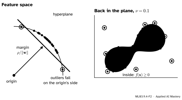
Step 2. A boundary in feature space. The one-class SVM of Schölkopf and colleagues uses the kernel trick (ML02.8). With the RBF kernel, \({k(\vect{x}, \vect{x}) = 1}\) for every point, so every mapped point lies at distance 1 from the origin of feature space, and since all kernel values are positive they lie on one side of it. The SVM separates the data from the origin with the widest margin it can, allowing a few points on the origin’s side.
ML03.9.4-F2
Left: with an RBF kernel every point sits on a sphere around the origin. A hyperplane cuts off the cap where the data crowd; points on the origin’s side are outliers. Right: the same boundary seen back in the plane.
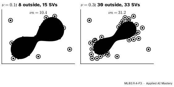
Step 3. The knob nu. The parameter \(\nu\) in \((0, 1]\) trades a tight boundary against the points it leaves outside: at most a share \(\nu\) of the training points may fall outside, and at least a share \(\nu\) become support vectors.
ML03.9.4-F3
With 104 training points, \({\nu = 0.1}\) leaves 8 outside (at most 10.4 allowed) and \({\nu = 0.3}\) leaves 30 (at most 31.2). Each fit has at least \({\nu n}\) support vectors.
Step 4. Judge with the labels you have. Fit each detector with no labels, rank the points by its score, and only then look at the known anomalies. The question is how high the detector put them.
The formal statement
PCA error, written out. Let \(\vect{q}_1, \dots, \vect{q}_d\) be the orthonormal principal directions and \({y_j = \vect{q}_j\T(\vect{x} - \bar{\vect{x}})}\). Then \({\vect{x} - \bar{\vect{x}} = \sum_{j=1}^{d} y_j \vect{q}_j}\) and the reconstruction keeps the first \(q\) terms, so
the second line because the \(\vect{q}_j\) are orthonormal. The score is the energy in the discarded directions; its average over the training data is the sum of the discarded eigenvalues (ML03.5.1).
The one-class SVM. With a feature map \(\phi\) and \(n\) training points, Schölkopf et al. (equations 4 to 6 of the report) solve
subject to \({\vect{w}\T\phi(\vect{x}_i) \ge \rho - \xi_i}\) and \({\xi_i \ge 0}\) for every \(i\), and flag a point when \({f(\vect{x}) = \vect{w}\T\phi(\vect{x}) - \rho}\) is negative. Each slack \(\xi_i\) lets a point fall short of the hyperplane at a price; \(\nu\) sets the price. Through the dual, \({f(\vect{x}) = \sum_i \alpha_i k(\vect{x}_i, \vect{x}) - \rho}\), a weighted sum of kernel bumps on the support vectors. With \({\nu = 1}\) every weight is \({1/n}\) and \(f\) is a thresholded kernel density estimate (ML03.8), section 3 of the report notes.
NoteResult: the nu-property (Proposition 4 of the report)
If \({\rho \ne 0}\), then \(\nu\) is an upper bound on the share of training points outside the boundary and a lower bound on the share of support vectors.
Judging a ranking. Rank \(N\) points by score, of which \(m\) are anomalies. Precision at \(k\) is the share of anomalies among the top \(k\). Let the anomalies sit at ranks \({r_1 < r_2 < \dots < r_m}\). When the \(j\)-th is reached, recall is \(j/m\) and precision is \(j/r_j\). Average precision weights each precision by the step in recall, \({\text{AP} = \sum_n (R_n - R_{n-1}) P_n}\) in scikit-learn’s notation, which here is
The ROC AUC is the share of (anomaly, normal) pairs that the score orders correctly (ML01.7.3).
Why AUC flatters. Let \(b_j\) be the number of normal points ranked above the \(j\)-th anomaly. There are \(N - m\) normals, so it is ordered correctly against \({N - m - b_j}\) of them. Average over the \(m\) anomalies:
where \(\bar b\) is the mean of the \(b_j\). Solving for it, \({\bar b = (1 - \text{AUC})(N - m)}\).
The number that matters to the person checking alarms is \(\bar b\), the false alarms above a typical anomaly. AUC divides it by the number of normals, so the rarer the anomalies, the smaller the penalty. On 357 normal rows an AUC of 0.914 still means about 31 false alarms above a typical anomaly. Saito and Rehmsmeier (2015) make the same case: on imbalanced data the precision-recall plot, whose chance level is the share of positives, is the more informative one.
Worked example
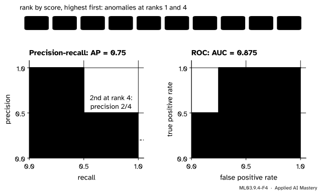
Ten points, two anomalies, ranked at 1 and 4.
ML03.9.4-F4
Average precision is the shaded area under the precision steps; AUC is the shaded area under the ROC staircase.
Precision at 2. The top two hold one anomaly: \({1/2 = 0.5}\).
Average precision. The first anomaly is found at rank 1 with precision \({1/1}\), the second at rank 4 with precision \({2/4}\):
ROC AUC. There are \({2 \times 8 = 16}\) (anomaly, normal) pairs. The anomaly at rank 1 is above all 8 normals; the one at rank 4 is above the 6 normals at ranks 5 to 10. So \({\text{AUC} = (8 + 6)/16 = 0.875}\), and \({\bar b = (1 - 0.875) \cdot 8 = 1}\): on average one false alarm above an anomaly, the normal points at ranks 2 and 3 shared between two anomalies.
Now make anomalies rare. Keep two anomalies, at ranks 1 and 50, among 1000 normals. The first is above all 1000 normals, the second above \({1000 - 48 = 952}\), so \({\text{AUC} = 1952/2000 = 0.976}\), which looks better than before. But \({\text{AP} = \tfrac12(\tfrac11 + \tfrac{2}{50}) = 0.52}\): by the time the second anomaly is found, 48 of the 50 alarms were false.
Result: precision at 2 is 0.5, AP 0.75 and AUC 0.875. Among 1000 normals, 48 false alarms above an anomaly still give AUC 0.976, while AP drops to 0.52.
Code
The PCA score from scratch on the twelve points, with \(q = 1\):
import numpy as npX = np.array([(1, 1), (2, 1), (1, 2), (2, 2), (3, 2), (6, 5), (7, 5), (6, 6), (7, 6), (8, 6), (4.5, 3.5), (9, 1)], dtype=float)mean = X.mean(axis=0)eigvals, Q = np.linalg.eigh(np.cov((X - mean).T))q1 = Q[:, [-1]] # the direction of largest varianceX_hat = mean + (X - mean) @ q1 @ q1.Terr = ((X - X_hat) **2).sum(axis=1)print("errors of bridge and (9, 1):", err[[10, 11]].round(3), " next largest:", np.sort(err)[-2].round(3))
errors of bridge and (9, 1): [ 0.047 18.33 ] next largest: 2.399
The one-class SVM and its \(\nu\)-property on the two blobs of the figures. Support vectors sit on the boundary, where the solver leaves values like \(10^{-7}\) of either sign, so a tight tolerance is set and a point counts as outside only when its value is below \(-10^{-4}\):
nu = 0.1: nu*n = 10.4, outside = 8, support vectors = 15
nu = 0.3: nu*n = 31.2, outside = 30, support vectors = 33
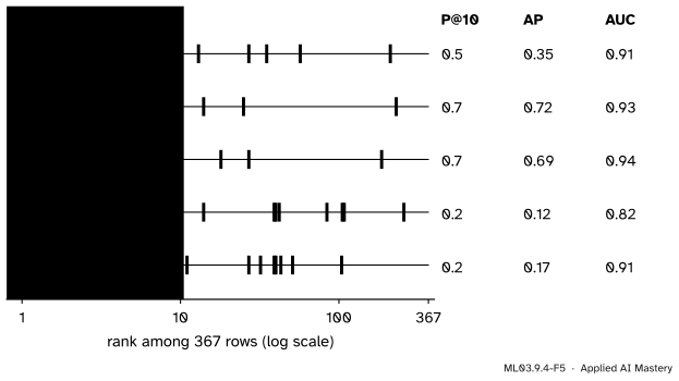
Now the contest. All 357 benign rows of load_breast_cancer and 10 malignant rows drawn with seed 0, standardised; five detectors with their library defaults, except \({q = 7}\) for PCA and \({\nu = 0.05}\) for the one-class SVM, fitted with no labels.
robust Mahalanobis   P@10 = 0.5   AP = 0.348   AUC = 0.910
LOF, k = 20          P@10 = 0.7   AP = 0.717   AUC = 0.931
isolation forest     P@10 = 0.7   AP = 0.691   AUC = 0.941
PCA error, q = 7     P@10 = 0.2   AP = 0.123   AUC = 0.818
one-class SVM        P@10 = 0.2   AP = 0.173   AUC = 0.914
ML03.9.4-F5
Where each detector ranks the ten planted malignant rows. AUC ranges only from 0.82 to 0.94; average precision ranges from 0.12 to 0.72, because it rewards what is at the top.
LOF and the isolation forest put 7 of the 10 in their top 10. The PCA error does worst: malignant tumours are larger (radius, area, perimeter), which moves them along the main directions of variation that PCA keeps, not off them. AUC hides most of these differences.
Explore
The module’s interactive is in ML03.9.3. Its contamination slider is precision at \(k\) in action: as you flag more points, watch how soon the flags stop landing on strays and start landing on the blobs.
Pitfalls
ML03.9.4-F6
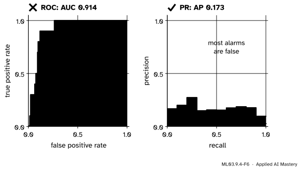
Wrong beside right, for the same detector on the same ranking. The ROC curve says 0.914. The precision-recall curve says that at every recall, most of the alarms are false.
“An AUC above 0.9 means the detector works.”
With 357 normal rows, an AUC of 0.914 still leaves about 31 false alarms above a typical anomaly. When anomalies are rare, report precision at the number of cases you can check, and average precision.
“Try settings until the ten labels look best.”
Ten labels are a tiny test set: tuning \(k\), \(\nu\) or \(q\) on them selects the luckiest setting, and the score you report is then optimistic. Fix settings before looking, or keep some labels aside to judge the final choice.
“The PCA error finds every strange point.”
It finds points off the subspace. A point far out along a principal direction is reconstructed well and scores low, like the bridge in the anchor figure and the large malignant tumours here. Pair it with a score inside the subspace, such as the Mahalanobis distance of \(\vect{y}\).
“Distances do not care about units.”
LOF, the one-class SVM with an RBF kernel and the PCA error all depend on scale; standardise features first (ML01.3.3). Two scores of this module are unaffected by rescaling a feature: the Mahalanobis distance (exercise 3 of ML03.9.1) and the isolation forest, whose thresholds are drawn uniformly over each feature’s own range and so stretch with it.
Check yourself
Recall
1. What is the PCA reconstruction-error score, in terms of the principal coordinates?
Show answer
\({e(\vect{x}) = \sum_{j > q} y_j^2}\): the squared length of the part of \({\vect{x} - \bar{\vect{x}}}\) in the discarded directions.
2. Why do all points lie on one sphere in the feature space of an RBF kernel?
Show answer
Because \({k(\vect{x}, \vect{x}) = \norm{\phi(\vect{x})}^2 = 1}\) for every point; and since every kernel value is positive, they all lie on the same side of the origin, which the one-class SVM cuts off with a hyperplane.
3. What does \(\nu\) bound in a one-class SVM?
Show answer
From above, the share of training points outside the boundary; from below, the share of support vectors (Proposition 4 of Schölkopf et al.).
4. Anomalies at ranks 1 and 4 of 10: give precision at 2, AP and AUC.
Show answer
Precision at 2 is 0.5; AP is \({\tfrac12(\tfrac11 + \tfrac24) = 0.75}\); AUC is \({(8 + 6)/16 = 0.875}\).
5. How many normal points does an AUC of 0.914 leave above a typical anomaly when there are 357 normal points?
Show answer
\({(1 - 0.914) \times 357 \approx 31}\).
Exercises
1.★ LOF ranks the ten malignant rows at 1, 2, 3, 5, 6, 7, 10, 14, 25 and 230. Compute its precision at 10 and its average precision.
Show solution
Seven ranks are 10 or less, so precision at 10 is 0.7. Average precision is the mean of \(j/r_j\):
which matches average_precision_score. The last anomaly, at rank 230, adds almost nothing.
2.★★ A detector puts all \(m\) anomalies directly after the first \(b\) normal points, among \(N - m\) normals. Find its AUC and its average precision. Evaluate both for \({m = 10}\), \({b = 10}\) and \({N - m = 357}\).
Show solution
Every anomaly has exactly \(b\) normals above it, so \({\text{AUC} = 1 - b/(N - m)}\). The \(j\)-th anomaly sits at rank \({b + j}\), so \({\text{AP} = \tfrac1m\sum_{j=1}^m \tfrac{j}{b + j}}\).
With the numbers:
\[
\begin{aligned}
\text{AUC} &= 1 - \tfrac{10}{357} = 0.972 , \\
\text{AP} &= \tfrac{1}{10}\big(\tfrac{1}{11} + \tfrac{2}{12} + \dots + \tfrac{10}{20}\big) \\
&= 0.331 .
\end{aligned}
\] Ten false alarms before the first real case barely dent AUC, but cut AP to a third.
3.★★★ Show that the PCA error of a point equals its squared distance to the subspace through \(\bar{\vect{x}}\) spanned by \(\vect{q}_1, \dots, \vect{q}_q\), so that no other point of that subspace is closer.
Show solution
Any point of the subspace is \({\vect{v} = \bar{\vect{x}} + \sum_{j \le q} b_j\vect{q}_j}\). With \({\vect{x} - \bar{\vect{x}} = \sum_{j=1}^{d} y_j\vect{q}_j}\):
The second sum does not depend on \(\vect{v}\), and the first is at least 0, with equality exactly when \({b_j = y_j}\) for every \({j \le q}\), which is the reconstruction \(\hat{\vect{x}}\). So the smallest squared distance is \({\sum_{j>q} y_j^2 = e(\vect{x})}\).
Summary card
Reconstruct, or draw a boundary; then judge by what lands at the top of the list.
ML03.9.4-F1
Off the subspace is strange.
PCA error.\({e(\vect{x}) = \norm{\vect{x} - \hat{\vect{x}}}^2 = \sum_{j>q} y_j^2}\); blind along the kept directions.
One-class SVM. Separate the data from the origin in feature space; \(\nu\) caps the share outside.
AP.\({\tfrac1m\sum_j j/r_j}\); P@k: anomalies in the top \(k\), over \(k\).
On breast cancer. LOF and isolation forest AP about 0.7; PCA error and one-class SVM below 0.2; all AUC 0.82 to 0.94.
Sources and next steps
Sources. Each was opened and checked against this lesson on 15 November 2026.
Bernhard Schölkopf, John C. Platt, John Shawe-Taylor, Alex J. Smola and Robert C. Williamson, Estimating the support of a high-dimensional distribution, Microsoft Research technical report MSR-TR-99-87, later published in Neural Computation 13(7), 2001. Section 3 gives the primal problem (equations 4 and 5), the decision function (6) and its kernel expansion (10), and notes that \(\nu = 1\) gives a Parzen windows estimate; section 5 shows that with a Gaussian kernel all mapped points have unit length in one orthant, and states the \(\nu\)-property as Proposition 4.
scikit-learn developers, sklearn.svm.OneClassSVM (nu as an upper bound on training errors and a lower bound on support vectors, gamma="scale") and sklearn.metrics.average_precision_score (AP as \({\sum_n (R_n - R_{n-1}) P_n}\), without interpolation). The User Guide, section 2.7 notes that the one-class SVM is sensitive to outliers in its training data.
Next. Anomalies in time series, with context and runs, are S07.10, and fraud in transactions is A08.1. Within this course, ML03.10, Evaluating clusters and embeddings, asks the same honest question of clusters and embeddings: is the structure an algorithm reports really in the data?