Read a factorisation as probabilities: a document picks a topic, the topic picks a word. Fit both tables by EM exactly as for a Gaussian mixture, work two iterations by hand, and see why the model is NMF with the Kullback-Leibler loss.
ML03.7.3L2 Intermediate25 minIn review (what this means)
The maths and code on this page are checked by automated tests on every change, but an independent reader has not signed it off yet. Spot a mistake or a confusing step? Tell us.
Write the probabilistic LSA model P(w | d) as a sum over topics and as a product of two probability tables.
Derive the E-step responsibilities and the M-step updates from expected counts, with Lagrange multipliers.
Carry out two EM iterations by hand and confirm that the log-likelihood rises.
Show that maximising the pLSA likelihood is minimising NMF’s Kullback-Leibler divergence, and explain why pLSA overfits.
The question
NMF said that d7, “team bake ball flour”, takes about 2.3 words from a sports part and 2.3 from a baking part. But 2.3 of what, and how sure is it? If a topic is a probability distribution over words and a document a probability distribution over topics, the corpus gets a likelihood, and the whole toolkit of maximum likelihood and EM from the Gaussian mixtures of ML03.4 applies.
From the last lesson
1. Write the multiplicative update for \(\mat{H}\) in NMF and say why it keeps entries non-negative.
Show answer
\({\mat{H} \leftarrow \mat{H} \circ (\mat{W}\T\mat{X}) / (\mat{W}\T\mat{W}\mat{H})}\). Each entry is multiplied by a ratio of non-negative numbers, so it cannot change sign.
2. Two NMF runs give different \(\mat{W}\). Name two reasons that do not mean either is wrong.
Show answer
Scaling (\({\mat{W}\mat{D}}\) with \({\mat{D}^{-1}\mat{H}}\) has the same product) and the order of the parts. Different starts can also reach different local minima.
Intuition
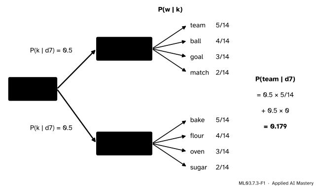
Tell a story of how each word of a document was written. The document has its own topic shares, \({P(k \mid d)}\). For each word, it first picks a topic \(k\) with those shares, and the topic then picks a word \(w\) with its own word probabilities \({P(w \mid k)}\).
ML03.7.3-F1
How pLSA explains a word of d7. The document picks a topic, half and half, and the topic picks a word. These are the fitted values on the corpus.
This is probabilistic latent semantic analysis (pLSA), Hofmann’s aspect model. The topic is latent: we see the words, never the topic that chose them. To find the probability of one word in d7, add up the routes to it. “Team” can only come from the sports topic, so \(P(\text{team} \mid d_7) = {0.5 \times 5/14} + {0.5 \times 0} = 0.179\).
Build it up
Step 1. One word, two routes. By the rule of total probability, summing over the topic,
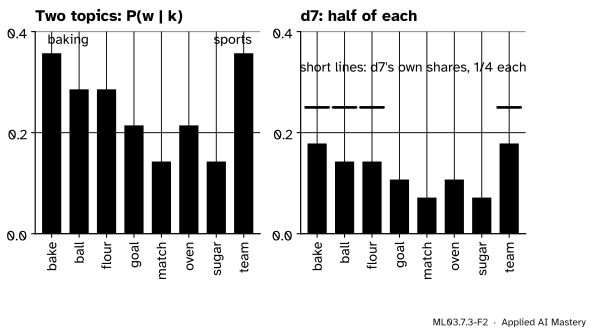
Step 2. It is a matrix product. Put the word probabilities of the topics into a \({V \times K}\) matrix and the topic shares of the documents into a \({K \times D}\) matrix. Then the table of \({P(w \mid d)}\) is their product, and every column of all three tables sums to 1. This is NMF with probability columns.
ML03.7.3-F2
\({P(w \mid d_7)}\) is half of each topic’s distribution. It cannot match d7’s own shares of 1/4 exactly, because both topics must also explain the other six documents.
Step 3. The likelihood. If word \(w\) occurs \({n(d, w)}\) times in document \(d\), the log-likelihood of the corpus is
Step 4. A logarithm of a sum. Setting the derivatives of \(\ell\) to zero gives no closed form, for the same reason as in a Gaussian mixture: the logarithm sits outside the sum over the latent topic. EM gets round it. If we knew which topic wrote each word, counting would do; since we do not, we count with probabilities.
The formal statement
NoteEM for pLSA
E-step. For every document \(d\) and word \(w\) with \({n(d, w) > 0}\), the responsibility of topic \(k\) is
where \({n_d = \sum_w n(d, w)}\) is the length of document \(d\). Each iteration leaves \(\ell\) the same or higher.
The E-step is Bayes’ rule. Given that the word in \(d\) is \(w\), the probability that topic \(k\) wrote it is the prior share \({P(k \mid d)}\) times the likelihood \({P(w \mid k)}\), divided by the total \({P(w \mid d)}\).
The M-step, derived. Fix the responsibilities, and write \({c_{dwk} = n(d, w)\,r_{dwk}}\) for the expected number of times word \(w\) in document \(d\) was written by topic \(k\). EM maximises the expected log-likelihood of the words and their topics,
Setting it to zero gives \({P(w \mid k) = \sum_d c_{dwk} / \lambda_k}\). Summing over \(w\) and using the constraint, \({\lambda_k = \sum_{w, d} c_{dwk}}\): the expected number of words written by topic \(k\). The same steps with the constraint \({\sum_k P(k \mid d) = 1}\) give a multiplier \(\sum_{k, w} c_{dwk} = n_d\), because the responsibilities of each word sum to 1. That the likelihood never falls is the general EM argument of ML03.4.3 (a lower bound that the E-step makes tight and the M-step raises).
The link to NMF. Lee and Seung’s second loss for NMF is the generalised Kullback-Leibler divergence
Take \({w_{wk} = P(w \mid k)}\) and \({h_{kd} = n_d\,P(k \mid d)}\). Then \({(\mat{W}\mat{H})_{wd} = n_d\,P(w \mid d)}\), and since each \({P(\cdot \mid d)}\) sums to 1, the product’s entries add up to \({\sum_d n_d}\), the same total as \(\mat{X}\). The last two terms cancel, and
where \({c = \sum_{w,d} x_{wd}\ln x_{wd} - \sum_d n_d \ln n_d}\) is fixed by the data. (The second line splits the logarithm of a product, and \({\sum_w x_{wd} = n_d}\).)
So minimising the divergence over such factors is maximising the pLSA likelihood. On the corpus, the KL-loss NMF of the last lesson split d7 into 2 and 2 words; pLSA gives it shares 0.5 and 0.5.
Worked example
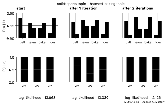
Two EM iterations on the small piece. Words ball, team, bake, flour; documents d2 = (1, 2, 0, 0), d5 = (0, 0, 2, 1) and d7 = (1, 1, 1, 1). Start with topic 1 leaning to sport, \({P(w \mid 1) = (0.4, 0.3, 0.2, 0.1)}\), topic 2 the reverse, \({(0.1, 0.2, 0.3, 0.4)}\), and every document at \({P(k \mid d) = 0.5}\). Then \({P(w \mid d) = 0.25}\) for every word, and \({\ell = 10\ln 0.25 = -13.863}\).
ML03.7.3-F3
Two EM iterations. The topics sharpen, d2 and d5 move towards their own topic, d7 stays at one half, and the log-likelihood climbs.
Iteration 1, E-step. All shares are 0.5, so they cancel and the responsibility of topic 1 is \({P(w \mid 1) / (P(w \mid 1) + P(w \mid 2))}\): 0.8 for ball, 0.6 for team, 0.4 for bake, 0.2 for flour.
Iteration 1, M-step. Expected counts for topic 1: ball \({0.8 + 0.8 = 1.6}\) (once in d2, once in d7), team \({2(0.6) + 0.6 = 1.8}\), bake \({2(0.4) + 0.4 = 1.2}\), flour \({0.2 + 0.2 = 0.4}\), in all 5.0. So \({P(w \mid 1) = (0.32, 0.36, 0.24, 0.08)}\), and by the same counts with \({1 - r}\), \({P(w \mid 2) = (0.08, 0.24, 0.36, 0.32)}\). The shares are each document’s topic-1 count over its length:
and in the same way 0.75 for team in d2, 0.25 for bake and 0.111 for flour in d5. In d7 the shares are still equal, so its responsibilities stay 0.8, 0.6, 0.4, 0.2.
Iteration 2, M-step. Topic 1’s counts are ball \({0.889 + 0.8 = 1.689}\), team \({2(0.75) + 0.6 = 2.1}\), bake \({2(0.25) + 0.4 = 0.9}\), flour \({0.111 + 0.2 = 0.311}\), again 5.0 in all, so \({P(w \mid 1) = (0.338, 0.42, 0.18, 0.062)}\). The shares become 0.796 for d2, 0.204 for d5 and still 0.5 for d7, and \({\ell = -12.126}\). Run on, the piece settles with d2 and d5 each in one topic and d7 shared equally, at \({\ell = -9.503}\).
Code
From scratch on the whole corpus: EM from several random starts.
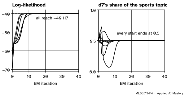
import numpy as npdocs = ["ball goal team goal", "team match ball team", "goal match team ball","flour sugar bake oven", "bake oven flour bake", "sugar flour bake oven","team bake ball flour"]words =sorted({w for d in docs for w in d.split()})N = np.array([[d.split().count(w) for d in docs] for w in words], dtype=float) # n(d, w), words x docsdef plsa(N, K, steps, seed): rng = np.random.default_rng(seed) Pwk = rng.uniform(size=(N.shape[0], K)) Pwk /= Pwk.sum(axis=0) # P(w | k): columns sum to 1 Pkd = np.full((K, N.shape[1]), 1/ K) # P(k | d): columns sum to 1for _ inrange(steps): ratio = np.divide(N, Pwk @ Pkd, out=np.zeros_like(N), where=N >0) counts = Pwk[:, :, None] * Pkd[None, :, :] * ratio[:, None, :] # n(d,w) r_dwk Pwk = counts.sum(axis=2) / counts.sum(axis=(0, 2)) Pkd = counts.sum(axis=0) / N.sum(axis=0) loglik = (N * np.log(np.where(N >0, Pwk @ Pkd, 1))).sum()return Pwk, Pkd, loglikruns = [plsa(N, 2, 500, seed) for seed inrange(5)]Pwk, Pkd, loglik = runs[0]sport =int(np.argmax(Pwk[words.index("team")]))print("log-likelihoods:", [round(float(r[2]), 3) for r in runs])print("sports topic x 14:", {w: round(float(v), 2) for w, v inzip(words, 14* Pwk[:, sport])})print("d7's topic shares:", Pkd[:, 6].round(4))
EM on the whole corpus from six random starts. The log-likelihood only rises and every start reaches the same maximum, where d7 is shared equally.
Each topic has 14 words’ worth of mass: the 12 words of its three documents plus two of d7’s four. The same answer comes from NMF with the Kullback-Leibler loss, once its parts are scaled to sum to 1:
from sklearn.decomposition import NMFkl = NMF(n_components=2, init="nndsvda", beta_loss="kullback-leibler", solver="mu", max_iter=5000, tol=1e-12, random_state=0).fit(N.T)parts = (kl.components_ / kl.components_.sum(axis=1, keepdims=True)).T # words x 2order = [int(np.argmax(parts[words.index("team")])), int(np.argmax(parts[words.index("bake")]))]print("largest gap to pLSA's topics:", np.abs(parts[:, order] - Pwk[:, [sport, 1- sport]]).max().round(4))
largest gap to pLSA's topics: 0.0
Explore
The module’s interactive, the factor explorer, sits in lesson ML03.7.2. Run NMF at rank 2 and compare its parts with the topics above: the same words lead each one.
Pitfalls
ML03.7.3-F5
Wrong beside right. If each document must come from one topic, d7’s baking words have to be explained by the sports topic. Letting each document mix topics fits better.
“A topic model is a clustering of documents.”
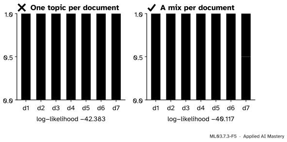
A clustering gives each document one group, so all its words come from one distribution. pLSA gives each word its own topic, and a document a mixture. Hofmann draws exactly this line between his aspect model and clustering models. On the corpus the best one-topic-per-document fit has log-likelihood \(-42.383\); the mixture reaches \(-40.117\) (it also has seven more parameters, the shares).
“pLSA can score a new document.”
\({P(k \mid d)}\) exists only for the documents it was trained on: \(d\) is an index into the training set. Blei, Ng and Jordan point out that pLSA is therefore not a generative model of documents, and that its \({KV + KD}\) parameters grow with the number of documents, which invites overfitting. To use it on a new document one must fit that document’s shares with the topics frozen, on the very words one wanted to score. The next lesson repairs this with a prior on the shares.
“EM found the topics, so they are the best ones.”
EM climbs to a local maximum. On this tiny corpus every start reaches \(-40.117\), but on real text different starts give different topics; run several and keep the highest likelihood.
3. How does the M-step re-estimate \({P(k \mid d)}\)?
Show answer
As the expected number of words of \(d\) written by topic \(k\), \({\sum_w n(d, w)\,r_{dwk}}\), divided by the length \(n_d\).
4. Which NMF loss matches the pLSA likelihood, and how are the factors related?
Show answer
The generalised Kullback-Leibler divergence, with \({w_{wk} = P(w \mid k)}\) and \({h_{kd} = n_d\,P(k \mid d)}\).
5. What are the fitted topic shares of d7 on the corpus, and why?
Show answer
0.5 and 0.5. Two of its four words (team, ball) only occur in the sports topic and two (bake, flour) only in the baking topic.
Exercises
1.★ With the fitted corpus model (d1 entirely sports; sports topic ball 4/14, goal 3/14, match 2/14, team 5/14), find \({P(w \mid d_1)}\) for each of d1’s words and the log-likelihood of d1, “ball goal team goal”.
Show solution
\({P(\text{ball} \mid d_1) = 4/14}\), \({P(\text{goal} \mid d_1) = 3/14}\), \({P(\text{team} \mid d_1) = 5/14}\). The log-likelihood is
2.★★ In the worked example after iteration 1, compute the responsibility of topic 1 for “team” in d2 and for “bake” in d5 (the values 0.75 and 0.25 used in iteration 2).
Show solution
In d2 the shares are \({(2/3, 1/3)}\) and team has \({P(\text{team} \mid k) = (0.36, 0.24)}\):
In d5 the shares are \({(1/3, 2/3)}\) and bake has \({(0.24, 0.36)}\): \({r = 0.08/(0.08 + 0.24) = 0.25}\).
3.★★★ Count the free parameters of pLSA with \(K\) topics, \(V\) words and \(D\) documents, and evaluate it for the corpus with \({K = 2}\). Compare with the number of words in the corpus.
Show solution
Each topic is a distribution over \(V\) words, with \({V - 1}\) free numbers; each document’s shares have \({K - 1}\). In all \({K(V - 1) + D(K - 1)}\). For the corpus, \({2 \times 7 + 7 \times 1 = 21}\) parameters for only 28 words. The second term grows with every new document, which is the overfitting that Blei, Ng and Jordan describe (they count \({KV + KD}\), without removing the sum-to-one constraints).
Same as NMF with the Kullback-Leibler loss; but no shares for unseen documents.
Sources and next steps
Sources. Each was opened and checked against this lesson on 15 November 2026.
T. Hofmann, Probabilistic Latent Semantic Analysis, UAI 1999. Section 3.1, equation 1: \({P(w \mid d) = \sum_z P(w \mid z) P(z \mid d)}\); section 3.2, equations 3 to 6: the E-step and the M-step proportional to expected counts (written there for the equivalent form \({P(z)\,P(d \mid z)\,P(w \mid z)}\), eq. 2); section 3.3: pLSA as a matrix product compared with LSA; section 3.5: aspects against clusters.
D. M. Blei, A. Y. Ng and M. I. Jordan, Latent Dirichlet Allocation, JMLR 3 (2003), 993 to 1022. Section 4.3: \(d\) is a dummy index into the training set, so pLSI is not a well-defined generative model of documents, and its \({kV + kM}\) parameters grow linearly with the number of documents.