Approximate a data matrix by a thin matrix times a wide one. The truncated SVD gives the best such product, and on a tiny corpus it becomes latent semantic analysis: words and documents in one plane, compared by angle.
ML03.7.1L2 Intermediate25 minIn review (what this means)
The maths and code on this page are checked by automated tests on every change, but an independent reader has not signed it off yet. Spot a mistake or a confusing step? Tell us.
Write a data matrix as an approximate product W H with inner dimension q, and read each column as a mix of q prototypes.
Use the Eckart-Young theorem to take the best rank-q product from the SVD, and compute the share of the sum of squares it keeps.
Fold a document into the reduced space by dot products and compare documents by cosine similarity, by hand and in code.
Run latent semantic analysis with TruncatedSVD on counts and on TF-IDF weights, and explain why its factors are hard to read.
The question
“Ball goal team goal” and “team match ball team” share two of their four words. “Goal match” shares only one word with each. A search engine that counts shared words calls these pairs weakly related, yet a person sees one subject in all three. Can a table of word counts discover, with no dictionary, that goal, match, ball and team belong together?
Intuition
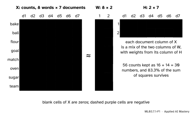
Write the corpus of this module as a table: one row per word, one column per document, and in each cell the number of times the word appears. Seven short documents over eight words give an 8 by 7 table of 56 counts. Most of it is predictable. Three documents talk about sport, three about baking, and one mixes both. Two “prototype” columns, a sports profile and a baking profile, could almost rebuild the table if each document said how much of each prototype it holds.
ML03.7.1-F1
The corpus as a product. An 8 by 7 table of counts is close to a thin 8 by 2 matrix times a wide 2 by 7 one, both of factors. Here \(\mat{W}\) and \(\mat{H}\) come from the SVD.
That is the whole idea of matrix factorisation: approximate a data matrix by the product of a thin matrix and a wide one. The thin matrix holds a few prototypes. The wide one says how much of each prototype every example uses. For text, this step is called latent semantic analysis (LSA), and it is how words that never appear together can still be found to belong together.
Build it up
Step 1. The shapes. Let \(\mat{X}\) be a \(V \times D\) matrix: \(V\) words, \(D\) documents. Choose a small inner dimension\(q\). We look for
Column \(d\) of the product is \(\mat{W}\vect{h}_d\), where \(\vect{h}_d\) is column \(d\) of \(\mat{H}\). So each document is approximated by a mix of the \(q\) columns of \(\mat{W}\), with weights \(\vect{h}_d\). Read by rows instead, each word is a mix of the \(q\) rows of \(\mat{H}\). In most data sets the examples are rows; here the documents are columns, because that is how a term-document matrix is written, and scikit-learn will want the transpose.
Step 2. The saving. The table has \({V D = 56}\) numbers. The factors with \({q = 2}\) have \({V q + q D = 16 + 14 = 30}\). For a real corpus, with 50,000 words, a million documents and \({q = 300}\), the saving is a factor of more than 150.
Step 3. How good is a product? Measure the squared error over every cell, the squared Frobenius norm of the difference:
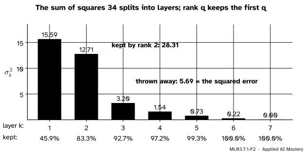
Step 4. The SVD splits the sum of squares into layers. Write the SVD as \({\mat{X} = \mat{U}\mat{\Sigma}\mat{V}\T}\), with singular values \({\sigma_1 \ge \sigma_2 \ge \dots}\). Then \(\mat{X}\) is a sum of rank-one layers \({\sigma_k \vect{u}_k \vect{v}_k\T}\) (M03.5.4), and the sum of squares of all entries is \({\sum_k \sigma_k^2}\) (derived below). For the corpus that total is 34: of its 28 words, six sit in three cells that hold a 2 and the other 22 sit in cells that hold a 1, so the sum of squares is \({22 + 3 \times 4 = 34}\). Rank \(q\) keeps the first \(q\) layers.
ML03.7.1-F2
The sum of squares 34 split into layers. The first two layers keep \({15.59 + 12.71 = 28.31}\) of it, 83.3 percent; the rest is the error of the best rank-2 product.
The last singular value is exactly 0. Documents d4 and d6 use the same four words once each, so their columns are equal and the matrix has rank 6, not 7. A bag of words cannot tell them apart.
The formal statement
NoteTheorem: the best product of a given inner dimension (Eckart and Young)
Let \({\mat{X} = \mat{U}\mat{\Sigma}\mat{V}\T}\) and keep the first \(q\) singular triples. Among all \(\mat{W}\) with \(q\) columns and \(\mat{H}\) with \(q\) rows, the squared error is smallest for
and the smallest error is the sum of the discarded squared singular values, \({\sum_{k > q} \sigma_k^2}\).
A product \(\mat{W}\mat{H}\) with \(q\) columns in \(\mat{W}\) has rank at most \(q\), so the theorem is the best rank-\(q\) approximation of M03.6.1, proved there. Two steps are new here, and each takes one line.
Why \(\mat{H}\) is also \(\mat{U}_q\T\mat{X}\). The columns of \(\mat{U}\) are orthonormal, so \(\mat{U}_q\T\mat{U}\) is the identity in its first \(q\) columns and zero after. Then
So the coordinates of document \(d\) are simply its dot products with the \(q\) columns of \(\mat{U}_q\): \({\vect{h}_d = \mat{U}_q\T \vect{x}_d}\). That gives a way to place a new document, or a search query, in the same space: take its count vector and multiply. This is called folding in.
Why the total is \({\sum_k \sigma_k^2}\). The squared Frobenius norm is the trace of \(\mat{X}\T\mat{X}\), and
using \({\operatorname{tr}(\mat{A}\mat{B}) = \operatorname{tr}(\mat{B}\mat{A})}\) and \({\mat{V}\T\mat{V} = \mat{I}}\). The share kept by rank \(q\) is \({\sum_{k \le q} \sigma_k^2 \big/ \sum_k \sigma_k^2}\).
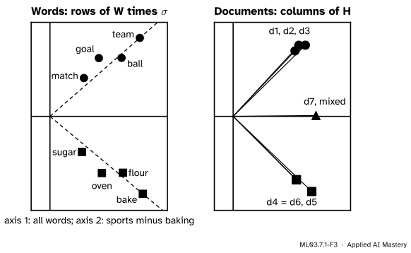
The corpus in the plane. With \({q = 2}\) every word and every document becomes a point in a plane. Words are the rows of \(\mat{U}_2\) (scaled by \(\sigma\)), documents the columns of \(\mat{H}\).
ML03.7.1-F3
Latent semantic analysis of the corpus. Sports words and baking words fall on two separate rays, the documents follow their words, and the mixed d7 sits between the two groups.
The first axis has positive weight on every word: it measures how long a document is. The second axis is “sports minus baking”. Neither axis is a topic; the topics are the two rays. Goal and match meet in only one document, d3, yet they land on the same ray, because they share neighbours (ball and team).
Worked example
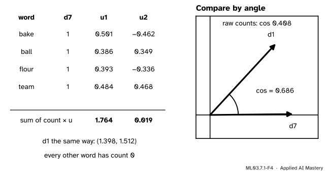
Fold d7 and d1 into the plane and compare them by angle. The first two columns of \(\mat{U}\), to three places, are listed for the words that d7 contains. (An SVD fixes each column only up to sign; we flip each so that its largest entry is positive.)
ML03.7.1-F4
Folding in is two dot products. d7’s four words add up their entries of \(\vect{u}_1\) and \(\vect{u}_2\); d1 does the same with its words. The angle between the results is the similarity.
Coordinates of d7. Its count vector has a 1 for bake, ball, flour and team and 0 elsewhere, so each coordinate is the sum of four entries:
The code below gets 1.512 for the second number, because it does not round the entries first.
Cosine. The cosine similarity of two vectors is their dot product divided by both lengths. The lengths are \({\sqrt{1.398^2 + 1.511^2} = 2.059}\) and \({\sqrt{1.764^2 + 0.019^2} = 1.764}\), and the two products in the dot product are \({1.398 \times 1.764 = 2.466}\) and \({1.511 \times 0.019 = 0.029}\), so
Unrounded, it is 0.686, an angle of about 47 degrees. On the raw counts the two documents share only ball and team, and their cosine is \({2 / (\sqrt{6} \times 2) = 0.408}\). The reduced space has pulled d7 halfway towards the sports group, which is fair: half of its words are sports words.
Code
From scratch: build the count matrix, take the SVD, fix the signs, and fold every document in.
import numpy as npdocs = ["ball goal team goal", "team match ball team", "goal match team ball","flour sugar bake oven", "bake oven flour bake", "sugar flour bake oven","team bake ball flour"]words =sorted({w for d in docs for w in d.split()})X = np.array([[d.split().count(w) for d in docs] for w in words], dtype=float) # 8 x 7U, s, Vt = np.linalg.svd(X, full_matrices=False)for k inrange(len(s)): # an SVD fixes signs only up to a flipif U[np.argmax(np.abs(U[:, k])), k] <0: U[:, k] *=-1 Vt[k] *=-1q =2W = U[:, :q]H = W.T @ X # fold in every document: H = U_q^T Xkept = (s[:q] **2).sum() / (X **2).sum()error = ((X - W @ H) **2).sum()def cosine(a, b):return a @ b / (np.linalg.norm(a) * np.linalg.norm(b))print(words)print("singular values:", s.round(3))print(f"sum of squares {(X **2).sum():.0f}, rank 2 keeps {kept:.1%}, error {error:.3f}")print("d7 at", H[:, 6].round(3), " d1 at", H[:, 0].round(3))print(f"cos(d1, d7): {cosine(H[:, 0], H[:, 6]):.3f} reduced, {cosine(X[:, 0], X[:, 6]):.3f} raw")print("negative cells in the rank-2 reconstruction:", int(((W @ H) <-1e-9).sum()))
['bake', 'ball', 'flour', 'goal', 'match', 'oven', 'sugar', 'team']
singular values: [3.949 3.566 1.788 1.242 0.853 0.474 0.   ]
sum of squares 34, rank 2 keeps 83.3%, error 5.692
d7 at [1.764 0.019]  d1 at [1.398 1.512]
cos(d1, d7): 0.686 reduced, 0.408 raw
negative cells in the rank-2 reconstruction: 12
The library route. CountVectorizer returns documents as rows, the transpose of our \(\mat{X}\), and TruncatedSVD returns each document’s coordinates, \({\mat{H}\T}\). Its default solver is randomised, so fix random_state, and compare signs loosely: a library may flip a column.
from sklearn.decomposition import TruncatedSVDfrom sklearn.feature_extraction.text import CountVectorizer, TfidfVectorizerfrom sklearn.metrics.pairwise import cosine_similaritycounts = CountVectorizer().fit_transform(docs) # 7 x 8, documents as rowslsa = TruncatedSVD(n_components=2, random_state=0)Z = lsa.fit_transform(counts)print("singular values:", lsa.singular_values_.round(3))print("cosines of d7 with d1..d6:", cosine_similarity(Z)[6, :6].round(3))tfidf = TfidfVectorizer().fit_transform(docs) # down-weights words in many documentsZt = TruncatedSVD(n_components=2, random_state=0).fit_transform(tfidf)C = cosine_similarity(Zt)print("TF-IDF: cos(d1, d2) =", C[0, 1].round(3), " cos(d1, d4) =", C[0, 3].round(3))
TF-IDF multiplies each count by a weight that is large for words found in few documents and small for words found everywhere, then scales each document to length 1. The scikit-learn guide recommends it over raw counts for LSA. On this corpus it changes little: the two groups stay apart.
Explore
The module’s interactive, the factor explorer, sits in lesson ML03.7.2. Set it to the SVD and step the rank from 1 to 4: the error falls exactly as the layers above predict, and purple cells mark the negative entries this lesson warned about.
Pitfalls
ML03.7.1-F5
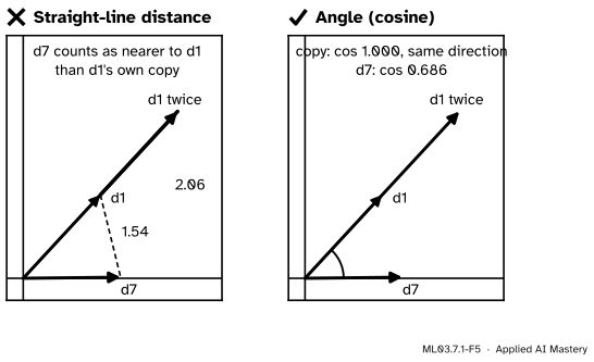
Wrong beside right. Writing d1 out twice doubles its arrow. Straight-line distance then calls the copy farther from d1 than the mixed d7 is; the angle sees that the copy says exactly the same thing.
“Nearest documents are the ones at the smallest distance.”
Distance mixes topic with length. A long document and a short one on the same subject point the same way but sit far apart. Compare by cosine, or scale every document to length 1 first, which TfidfVectorizer does by default.
“The second factor is the baking topic.”
The second column of \(\mat{U}\) is sports minus baking, and the first is all words at once. Any rotation of the two columns spans the same plane and fits just as well, so individual SVD factors carry no promise of meaning. Worse, they mix signs: the rank-2 reconstruction has 12 negative cells, such as \({-0.119}\) “oven” in d1, which no count can be. The next lesson fixes this by forbidding negative entries.
“explained_variance_ratio_ is the share that rank 2 keeps.”
TruncatedSVD does not centre the data, but its explained_variance_ratio_ measures the variance of each coordinate column. On the corpus it reports 0.010 and 0.684, not 0.459 and 0.374. The first axis, length, hardly varies between documents, so its variance is small even though it carries the most of the sum of squares. Compute \({\sigma_k^2 / \norm{\mat{X}}_F^2}\) yourself.
Check yourself
Recall
1. In \({\mat{X} \approx \mat{W}\mat{H}}\) with \(\mat{X}\) of size \({V \times D}\), what are the shapes of \(\mat{W}\) and \(\mat{H}\), and how is column \(d\) of \(\mat{X}\) approximated?
Show answer
\(\mat{W}\) is \({V \times q}\) and \(\mat{H}\) is \({q \times D}\). Column \(d\) is approximated by \(\mat{W}\vect{h}_d\), a mix of the \(q\) columns of \(\mat{W}\) with weights from column \(d\) of \(\mat{H}\).
2. What is the smallest squared error of a rank-\(q\) product, and which product reaches it?
Show answer
\({\sum_{k > q} \sigma_k^2}\), reached by \({\mat{W} = \mat{U}_q}\) and \({\mat{H} = \mat{\Sigma}_q\mat{V}_q\T}\) (Eckart and Young).
3. How is a new document placed in the reduced space?
Show answer
By folding in: multiply its count vector by \(\mat{U}_q\T\), which takes its dot product with each of the \(q\) columns of \(\mat{U}_q\).
4. What share of the corpus’s sum of squares does rank 2 keep, and why?
Show answer
83.3 percent: \({(15.59 + 12.71)/34 = 28.31/34}\), since the sum of squares is \({\sum_k \sigma_k^2}\).
5. Why is the corpus’s term-document matrix of rank 6 rather than 7?
Show answer
Documents d4 and d6 contain the same four words once each, so their columns are equal.
Exercises
1.★ What share of the sum of squares does rank 1 keep, and what is the squared error of the best rank-3 product?
Show solution
Rank 1 keeps \({15.59 / 34 = 45.9}\) percent. The best rank-3 error is the sum of the discarded squared singular values, which is the total minus the three that are kept: \({34 - (15.59 + 12.71 + 3.20) = 2.50}\) (2.495 unrounded), so rank 3 keeps 92.7 percent.
2.★★ A user searches for “goal match”. Fold the query into the plane with the entries of \(\vect{u}_1\) and \(\vect{u}_2\) (goal: 0.264, 0.347; match: 0.183, 0.229), and find its cosine with d2, whose coordinates are (1.538, 1.514). Compare with the cosine on raw counts.
Show solution
The query has goal 1 and match 1, so its first coordinate is \({0.264 + 0.183 = 0.447}\) and its second \({0.347 + 0.229 = 0.576}\). The two lengths are 0.729 and 2.158, with product 1.5732, and the products in the dot product are \({0.447 \times 1.538 = 0.6875}\) and \({0.576 \times 1.514 = 0.8721}\), so
On raw counts the query and d2 (“team match ball team”) share only “match”: the dot product is 1, the lengths are \(\sqrt{2}\) and \(\sqrt{6}\), and the cosine is \({1/\sqrt{12} = 0.289}\). LSA finds the match that word overlap misses.
3.★★★ Show that if every column of \(\mat{X}\) is multiplied by its own positive number (documents of different lengths), the cosine between two documents on raw counts does not change, but the LSA plane can. What does this say about normalising before the SVD?
Show solution
Cosine divides by both lengths: for \({a, b > 0}\), \({\cos(a\vect{x}, b\vect{y}) = ab\,\vect{x}\T\vect{y} / (a\norm{\vect{x}}\, b\norm{\vect{y}})}\), and \(a\) and \(b\) cancel. The SVD, though, minimises squared error over all cells, so a column multiplied by a large number weighs more in the fit and pulls the leading singular vectors towards itself; the plane, and so every reduced cosine, can change. Scaling every document to length 1 (as TfidfVectorizer does) before the SVD stops long documents from steering the factorisation.
Summary card
A thin matrix of prototypes times a wide matrix of weights.
ML03.7.1-F1
Rank 2 keeps 83.3 percent.
Factorisation:\({\mat{X} \approx \mat{W}\mat{H}}\), with \(\mat{W}\) of size \({V \times q}\) and \(\mat{H}\) of size \({q \times D}\).
Best in squared error:\({\mat{W} = \mat{U}_q}\), \({\mat{H} = \mat{U}_q\T\mat{X}}\); error \({\sum_{k>q}\sigma_k^2}\).
Fold in:\({\vect{h} = \mat{U}_q\T\vect{x}}\), then compare by cosine.
Sources and next steps
Sources. Each was opened and checked against this lesson on 15 November 2026.
T. Hofmann, Probabilistic Latent Semantic Analysis, UAI 1999. Section 2.2 describes LSA as an SVD of the co-occurrence table truncated to the largest \(K\) singular values, rank-\(K\) optimal in the \(L_2\) sense, with rows of \(\mat{U}\mat{\Sigma}\) as coordinates; section 3.3 notes that the LSA approximation may contain negative entries and that its directions have no obvious interpretation.
scikit-learn, TruncatedSVD: does not centre the data, defaults to the randomised solver, and defines explained_variance_ as the variance of the transformed training samples.