Run t-SNE from scratch with momentum and early exaggeration on 500 handwritten digits, match scikit-learn’s TSNE, and learn what a t-SNE picture cannot show: cluster sizes, gaps between clusters, and clumps in pure noise.
ML03.6.3L2 Intermediate30 minIn review (what this means)
The maths and code on this page are checked by automated tests on every change, but an independent reader has not signed it off yet. Spot a mistake or a confusing step? Tell us.
Implement t-SNE from scratch with gradient descent, momentum and early exaggeration, and compute one update by hand.
Run sklearn.manifold.TSNE with PCA initialisation and a fixed random_state, and judge a map by more than its look.
Explain how the perplexity changes a t-SNE map, using maps of the same data at perplexities 2 to 100.
State what a t-SNE map cannot show (cluster sizes, distances between clusters, structure in noise) and the cost of the exact method.
The question
The last lesson built the cost and its gradient. Now run it: 500 images of handwritten digits, 64 pixels each, laid out on a page. The picture that comes out is striking, ten islands with water between them. But how much of that picture is the data, and how much is the method? If one island is twice the size of another, or twice as far away, does that mean anything?
From the last lesson
1. How is the perplexity of a row defined?
Show answer
\({2^{H_i}}\), with \({H_i = -\sum_j p_{j|i}\log_2 p_{j|i}}\) the entropy of row \(i\) in bits: an effective number of neighbours.
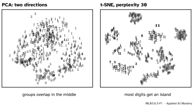
PCA (ML03.5) gives the best flat view of the digits: it keeps as much spread as two straight directions can. t-SNE does not look for a view at all. It moves 500 dots until each dot’s neighbours in the map are the ones it had among the images.
ML03.6.3-F1
The same 500 digits. Left: the two leading principal directions. Right: t-SNE with perplexity 30. Most digits get an island of their own; the ones split into two.
The price of that freedom is that the map’s geometry is invented to serve the neighbourhoods. Inside an island the order of the points means something. The size of an island and the space between islands mostly do not. This lesson builds the method and then learns to read it.
Build it up
Step 1. Start small. Place the \(n\) map points at random, very close to the origin (a normal distribution with standard deviation \(10^{-4}\), as scikit-learn does; the paper’s start has variance \(10^{-4}\)), or at the first two principal scores shrunk to that size.
Step 2. Step downhill with momentum. Each iteration computes the gradient \(\vect{g}\) of the last lesson and updates a velocity \(\vect{v}\) and the map:
The momentum\(\cparam{\alpha}\) keeps part of the last move, so the map keeps rolling in a direction the gradient keeps choosing. van der Maaten and Hinton use \({\alpha = 0.5}\) for the first 250 iterations and 0.8 after, 1000 iterations in all.
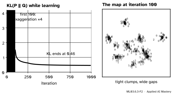
Step 3. Exaggerate early. For the first iterations, multiply every \(p_{ij}\) by a factor, 4 in the paper (12 in scikit-learn). The \(q_{ij}\) still add up to 1, so they cannot match the inflated \(p_{ij}\), and the cost pushes hard on the largest ones: neighbours are pulled into tight clumps with empty space between them, which the clumps can then move through to find their places.
ML03.6.3-F2
Training on 500 digits with perplexity 30. Left: the cost. During exaggeration it is measured against the true \(P\), so it stays high; it falls fast once the clumps are released. Right: the map at the end of exaggeration: tight clumps, wide gaps.
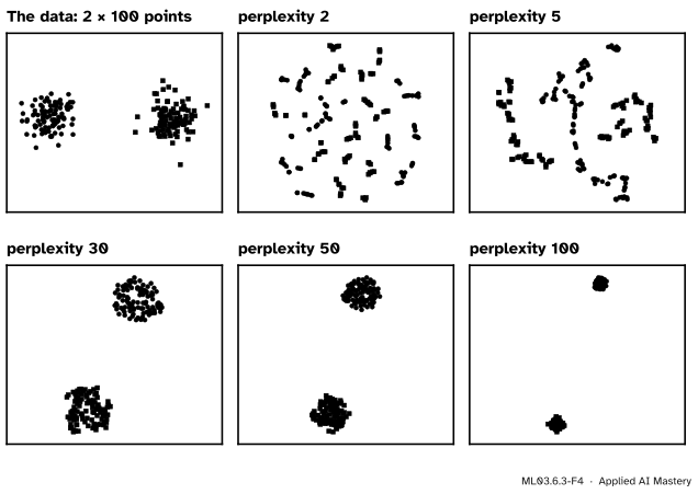
Step 4. Choose the perplexity. It sets the size of every neighbourhood, so it changes the picture more than anything else. The figure below shows two round clusters of 100 points under five perplexities.
ML03.6.3-F4
One dataset, five maps. At perplexity 2 each point sees one or two neighbours and the clusters shatter into fragments. From 30 on the two clusters appear; at 100, half the dataset, each point’s neighbourhood covers its whole cluster.
The formal statement
NoteAlgorithm: t-SNE with momentum and early exaggeration
Input: data \(\cdata{\vect{x}_1, \dots, \vect{x}_n}\), perplexity, iterations \(T\), learning rate \(\eta\), momentum \(\alpha_t\), exaggeration \(c\) for the first \(T_0\) iterations.
Compute \(p_{j|i}\) with the chosen perplexity and \({p_{ij} = (p_{j|i} + p_{i|j})/2n}\).
Draw \(\cmodel{\vect{y}_i}\) from a normal distribution with tiny variance; set \({\vect{v}_i = \vect{0}}\).
For \({t = 1, \dots, T}\): compute \(q_{ij}\); compute the gradient with \(c\,p_{ij}\) in place of \(p_{ij}\) while \({t \le T_0}\); set \({\vect{v} \leftarrow \alpha_t\vect{v} - \eta\,\vect{g}}\) and \({\vect{y} \leftarrow \vect{y} + \vect{v}}\).
Why momentum speeds things up. If the gradient stays the same, \(\vect{g}\), for several steps, the velocity after \(k\) steps is a geometric sum:
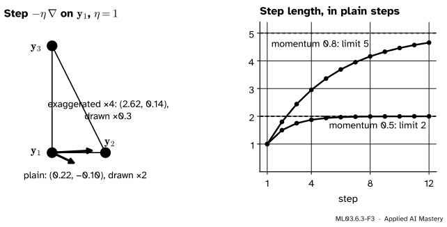
The step grows towards \({1/(1 - \alpha)}\) plain steps: 2 for \({\alpha = 0.5}\) and 5 for \({\alpha = 0.8}\). Where the gradient flips sign from step to step, the terms cancel instead, so the map speeds up along steady slopes and calms down across ravines.
The cost of exactness. Every iteration touches all \({n(n-1)}\) pairs: 249,500 for 500 points, but about 4.9 billion for 70,000 points. The Barnes-Hut approximation, scikit-learn’s default method='barnes_hut', treats a whole region of far-away points as a single point (the angle parameter sets how large a region may be), which brings the cost of an iteration down to about \({n\log n}\).
Worked example
One update by hand. Three map points \({\vect{y}_1 = (0, 0)}\), \({\vect{y}_2 = (1, 0)}\) and \({\vect{y}_3 = (0, 2)}\), with \({p_{12} = 0.4}\) and \({p_{13} = p_{23} = 0.05}\). Last lesson’s exercise gave \({q_{12} = 0.2885}\), \({q_{13} = 0.1154}\), \({q_{23} = 0.0962}\), from kernel values \({w_{12} = \tfrac12}\), \({w_{13} = \tfrac15}\), \({w_{23} = \tfrac16}\).
The gradient at \(\vect{y}_1\). One term per other point, \({4(p_{1j} - q_{1j})\,w_{1j}(\vect{y}_1 - \vect{y}_j)}\):
So \({\vect{g}_1 = (-0.2231, 0.1046)}\). With \({\eta = 1}\) and no momentum yet, \(\vect{y}_1\) moves by \({-\vect{g}_1 = (0.223, -0.105)}\): towards \(\vect{y}_2\), which is too far, and away from \(\vect{y}_3\), which is too close.
With exaggeration 4. Now \({p_{12} = 1.6}\) and \({p_{13} = 0.2}\), while the \(q\) stay the same:
The step \({(2.623, 0.135)}\) is almost eleven times longer, and the push from \(\vect{y}_3\) has become a pull: exaggerated, every real neighbour attracts.
Momentum. If the same plain gradient came back at the next step, the velocity would be
1.5 plain steps; then 1.75, then 1.875, approaching 2.
ML03.6.3-F3
Left: the step on \(\vect{y}_1\), plain and with exaggeration 4. Right: with a steady gradient, momentum 0.5 doubles the step and momentum 0.8 multiplies it by five.
Code
A from-scratch t-SNE in about twenty lines, run on 500 digits with perplexity 30, exaggeration 4 for 100 iterations and \({\eta = 100}\). A map has no units to check, so we judge it by a task: the accuracy of a 5-nearest-neighbour classifier in the map, under 5-fold cross-validation, against the same in the PCA view.
import numpy as npfrom sklearn.datasets import load_digitsfrom sklearn.decomposition import PCAfrom sklearn.model_selection import cross_val_scorefrom sklearn.neighbors import KNeighborsClassifierdef sq_dists(Z): s = (Z **2).sum(1)return np.maximum(s[:, None] + s[None, :] -2* Z @ Z.T, 0)def joint_probs(X, perplexity): D, n = sq_dists(X), len(X) P = np.zeros((n, n))for i inrange(n): d = np.delete(D[i], i) lo, hi, s =0.0, np.inf, 1.0for _ inrange(100): # binary search for sigma_i p = np.exp(-(d - d.min()) / (2* s * s)); p /= p.sum() h =2**-(p[p >0] * np.log2(p[p >0])).sum()ifabs(h - perplexity) <1e-5: break lo, hi = (lo, s) if h > perplexity else (s, hi) s = (lo + hi) /2if hi < np.inf else2* s P[i, np.arange(n) != i] = preturn (P + P.T) / (2* n)def tsne(P, iters=1000, lr=100.0, exaggeration=4.0, exag_iters=100, seed=0): Y = np.random.default_rng(seed).normal(0, 1e-4, (len(P), 2)) V = np.zeros_like(Y)for it inrange(iters): w =1/ (1+ sq_dists(Y)); np.fill_diagonal(w, 0) Q = w / w.sum() M = ((exaggeration if it < exag_iters else1.0) * P - Q) * w g =4* (M.sum(1)[:, None] * Y - M @ Y) V = (0.5if it <250else0.8) * V - lr * g Y = Y + V m = P >0return Y, (P[m] * np.log(P[m] / Q[m])).sum()X, labels = load_digits(return_X_y=True)pick = np.random.default_rng(0).choice(len(X), 500, replace=False)X, labels = X[pick], labels[pick]P = joint_probs(X, 30)Y, cost = tsne(P)knn = KNeighborsClassifier(5)acc_tsne = cross_val_score(knn, Y, labels, cv=5).mean()acc_pca = cross_val_score(knn, PCA(2).fit_transform(X), labels, cv=5).mean()print(f"from scratch: KL = {cost:.3f} 5-NN accuracy in the map {acc_tsne:.3f}, in the PCA view {acc_pca:.3f}")
from scratch: KL = 0.455 5-NN accuracy in the map 0.952, in the PCA view 0.662
The same with scikit-learn: PCA initialisation and a fixed random_state make the run repeatable, and a second seed shows how much a run can differ.
from scipy.spatial import procrustesfrom sklearn.manifold import TSNEruns = {"pca": TSNE(2, perplexity=30, init="pca", random_state=0).fit(X),"random": TSNE(2, perplexity=30, init="random", random_state=1).fit(X)}for name, model in runs.items(): acc = cross_val_score(knn, model.embedding_, labels, cv=5).mean()print(f"TSNE init={name}: KL = {model.kl_divergence_:.3f} 5-NN accuracy {acc:.3f}")gap = {"pca against random start": procrustes(runs["pca"].embedding_, runs["random"].embedding_)[2],"ours against TSNE": procrustes(Y, runs["pca"].embedding_)[2]}print("Procrustes disparity (0 = same up to turning and scaling):", {k: round(float(v), 3) for k, v in gap.items()})print("pairs per iteration, n = 500:", 500*499, " n = 70,000:", f"{70_000*69_999:.2e}")
TSNE init=pca: KL = 0.520   5-NN accuracy 0.954
TSNE init=random: KL = 0.521   5-NN accuracy 0.952
Procrustes disparity (0 = same up to turning and scaling): {'pca against random start': 0.003, 'ours against TSNE': 0.413}
pairs per iteration, n = 500: 249500   n = 70,000: 4.90e+09
Both starts reach the same cost, and scipy.spatial.procrustes, which turns, flips and scales one map onto the other, finds them almost identical: on these digits the layout is stable. Our own map, made with exaggeration 4 instead of 12 and another learning rate, is laid out differently (disparity about 0.4) though its neighbourhoods are as good. The arrangement of the islands depends on the settings, and Distill’s authors show data where even two seeds differ a lot. Note also that TSNE has fit and fit_transform but no transform: a new image cannot be placed on an existing map without running the whole optimisation again.
Explore
ML03.6-X1
Live t-SNE
Pick a preset and press play: t-SNE runs in the page, and the map on the right rearranges beside the data on the left. Slide the perplexity, switch early exaggeration off and on, and try the uniform noise at perplexity 2 against 30, watching the KL divergence in the read-out.
Pitfalls
ML03.6.3-F5
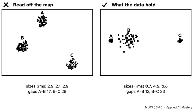
Wrong beside right. t-SNE gives the three clusters nearly equal sizes, 2.0, 2.1 and 2.0, though in the data B is more than five times wider than A. The far gap, almost three times the near one in the data, is less than twice it in the map.
“This cluster is bigger in the map, so it is more spread out in the data.”
Each \(\sigma_i\) adapts to the local density, so dense clusters are expanded and sparse ones shrunk. Wattenberg, Viégas and Johnson put it bluntly: cluster sizes in a t-SNE plot mean nothing. Measure spreads in the data.
“These islands are far apart, so the groups are very different.”
Distances between well-separated clusters may mean nothing; they also change with the perplexity. Here the data’s 12 and 33 became 17 and 28. Compare groups with distances in the original space, or with the measures of ML03.10.4.
ML03.6.3-F6
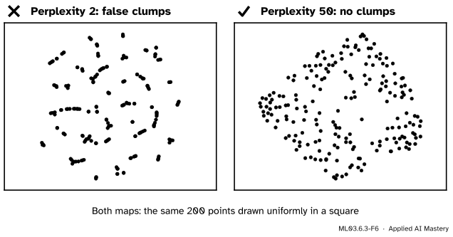
Pure noise. At perplexity 2 the map shows dozens of convincing little groups that are not in the data.
“The map shows clumps, so the data have clusters.”
At low perplexity t-SNE builds clumps out of uniform noise. Before believing a cluster, check that it survives several perplexities and seeds, and test it with the methods of ML03.10.3.
Check yourself
Recall
1. Write the momentum update of t-SNE.
Show answer
\({\vect{v} \leftarrow \alpha\vect{v} - \eta\vect{g}}\) and \({\vect{y} \leftarrow \vect{y} + \vect{v}}\), with \({\alpha = 0.5}\) early and 0.8 later in the original paper.
2. What does early exaggeration do, and why does it help?
Show answer
It multiplies every \(p_{ij}\) by a factor (4, or 12 in scikit-learn) for the first iterations, which pulls neighbours into tight, well-separated clumps that can move past each other to find a good global arrangement.
3. With a steady gradient, how long does a step become under momentum \(\alpha\)?
Show answer
After \(k\) steps, \({(1 - \alpha^k)/(1 - \alpha)}\) plain steps, approaching \({1/(1 - \alpha)}\): 2 for 0.5, 5 for 0.8.
4. Name three things a t-SNE map cannot be trusted to show.
Show answer
The relative sizes of clusters, the distances between well-separated clusters, and whether clumps are real (uniform noise forms clumps at low perplexity).
5. What does method='barnes_hut' change?
Show answer
It approximates the gradient by treating whole regions of far-away points as single points, so an iteration costs about \({n\log n}\) instead of \({n^2}\).
Exercises
1.★ In the worked example, compute the gradient at \(\vect{y}_3\) without exaggeration and say which way \(\vect{y}_3\) moves.
Show solution
Each term is \({4(p_{3j} - q_{3j})\,w_{3j}(\vect{y}_3 - \vect{y}_j)}\):
So \({\vect{g}_3 = (0.0308, -0.1662)}\) and \(\vect{y}_3\) moves by \({(-0.031, 0.166)}\): up and a little left, away from both, since both pairs are too close. The three gradients add up to zero, as the last lesson proved.
2.★★ A run of t-SNE on 2,000 points takes 4 seconds with the exact method. Estimate the exact time for 20,000 points, and say why Barnes-Hut changes the answer.
Show solution
The exact method costs about \(n^2\) per iteration. Ten times the points is a hundred times the work: about 400 seconds, nearly seven minutes, and a hundred times the memory for the \(n \times n\) matrices. Barnes-Hut costs about \({n\log n}\), so the factor is
3.★★★ Explain, using the perplexity search, why perplexity 2 shatters the two round clusters of the figure into fragments, and why perplexity 100 on 200 points makes each cluster small and tight.
Show solution
At perplexity 2, each \(\sigma_i\) shrinks until \(i\) spreads its probability over about two neighbours. Almost all of \(P\) then sits on pairs of nearest neighbours, and the cost only asks the map to keep those tiny groups together; nothing ties one tiny group to the next, so the clusters fall apart into fragments. At perplexity 100, each \(\sigma_i\) grows until about 100 points share the probability, which is a whole cluster. Every pair inside a cluster gets a similar, sizeable \(p_{ij}\), the map pulls each cluster into a tight ball, and the pairs across clusters, which carry almost no probability, are pushed far apart.
Summary card
t-SNE keeps neighbourhoods; sizes and gaps are its own invention.
Early exaggeration.\(p_{ij}\) times 4 (12 in scikit-learn) at first: tight clumps that can move.
Perplexity. 5 to 50 usually; always look at several.
Do not read cluster sizes, gaps between clusters, or clumps at low perplexity.
Cost.\(n^2\) exact; Barnes-Hut about \({n\log n}\); no transform for new points.
Sources and next steps
Sources. Each was opened and checked against this lesson on 15 November 2026.
Laurens van der Maaten and Geoffrey Hinton, Visualizing Data using t-SNE, JMLR 9 (2008). Algorithm 1 gives the simple version with momentum and the start from \({\mathcal{N}(0, 10^{-4}I)}\); Section 3.4 describes early exaggeration (“multiply all of the \(p_{ij}\)’s by, for example, 4”), and the settings used throughout: exaggeration 4 for the first 50 iterations, 1000 iterations, momentum 0.5 before iteration 250 and 0.8 after, and a learning rate that starts at 100 and is adapted during the run (the scheme of Jacobs, 1988).
Martin Wattenberg, Fernanda Viégas and Ian Johnson, How to Use t-SNE Effectively, Distill (2016). Sections on perplexity, “Cluster sizes in a t-SNE plot mean nothing”, “Distances between clusters might not mean anything” and “Random noise doesn’t always look random”, and the advice to look at several perplexities and runs.
scikit-learn 1.9, sklearn.manifold.TSNE (defaults perplexity 30, early_exaggeration 12, init ‘pca’, method ‘barnes_hut’ in \({O(N\log N)}\) against ‘exact’ in \({O(N^2)}\); kl_divergence_; no transform method) and User Guide Section 2.2.9, which notes that different seeds can give different embeddings.
Next.ML03.6.4 UMAP builds a map from a weighted neighbour graph again, trains it by sampling edges, and can place new points on an existing map.