Turn distances into neighbour probabilities, with a Gaussian whose width is set by the perplexity, and look for a map whose Student-t probabilities match them. Derive the t-SNE gradient line by line and read it as springs that pull and push.
ML03.6.2L2 Intermediate30 minIn review (what this means)
The maths and code on this page are checked by automated tests on every change, but an independent reader has not signed it off yet. Spot a mistake or a confusing step? Tell us.
Compute the conditional probabilities p_(j|i) of a point, their entropy and their perplexity, and find sigma_i by binary search.
Build the symmetric probabilities p_ij and the Student-t map probabilities q_ij, and explain how the heavy tail answers the crowding problem.
Derive the gradient of KL(P || Q) for t-SNE line by line and read it as springs that attract and repel.
Compute the affinities of ten points from scratch and check the gradient against finite differences.
The question
The eigenmap of the last lesson keeps neighbours together, but it has no reason to leave space between groups. A picture of 500 handwritten digits should show ten islands, one per digit, with water between them. What should a map try to match so that each point keeps the same neighbours, and how can it make room for the groups to separate?
From the last lesson
1. What eigenproblem gives the Laplacian eigenmap?
Show answer
\({\mat{L}\vect{y} = \lambda\mat{D}\vect{y}}\) with \({\mat{L} = \mat{D} - \mat{W}}\). The constant eigenvector, with \({\lambda = 0}\), is dropped and the next ones are the coordinates.
2. Why does a k-nearest-neighbour graph fail on the swiss roll when \(k\) is too large?
Show answer
Its edges reach across the gap between turns and short-circuit the sheet, so the embedding folds the turns together.
Intuition
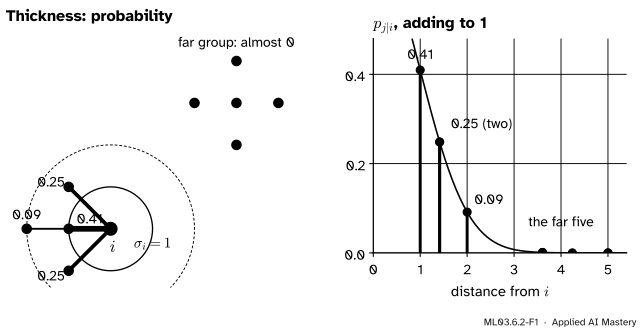
Imagine that point \(i\) picks one neighbour at random, favouring the near ones. The chance that it picks \(j\) is a number between 0 and 1, and the chances for all \(j\) add up to 1. Near points get a large share, far points almost nothing. That list of chances describes \(i\)’s neighbourhood without mentioning a single distance.
ML03.6.2-F1
Point \(i = (1, 0)\) of the ten points turns its distances into probabilities with a Gaussian of width \({\sigma_i = 1}\). Its own group gets 0.41, 0.25, 0.25 and 0.09; the five far points share less than 0.003.
SNE, stochastic neighbour embedding, computes these chances in the data, computes the same kind of chances between points of a map, and moves the map until the two sets of chances agree. t-SNE changes one thing: in the map it uses a curve with a much heavier tail than the Gaussian, which gives clusters room to pull apart.
Build it up
Step 1. Chances in the data. For each point \(i\), a Gaussian centred on \(\cdata{\vect{x}_i}\) gives the conditional probability that \(i\) picks \(j\):
with \(p_{i|i} = 0\). Each point has its own bandwidth \(\cparam{\sigma_i}\), because the data are denser in some places than others.
Step 2. Choose \(\sigma_i\) by perplexity. Small \(\sigma_i\) gives almost all the chance to the nearest point; large \(\sigma_i\) spreads it evenly. The spread is measured by the entropy in bits, \({H_i = -\sum_j p_{j|i}\log_2 p_{j|i}}\), and the perplexity is \({2^{H_i}}\). If \(i\) spread its chance evenly over \(m\) points the perplexity would be exactly \(m\), so it reads as an effective number of neighbours. The user fixes one perplexity for all points, typically between 5 and 50, and a binary search finds each \(\sigma_i\).
Step 3. Make it symmetric. Set \({p_{ij} = (p_{j|i} + p_{i|j})/2n}\). Now \({p_{ij} = p_{ji}}\), the \({n(n-1)}\) values add up to 1, and every point owns at least \({1/2n}\) of the total, so an outlier still matters.
Step 4. Chances in the map. For map points \(\cmodel{\vect{y}_i}\) in the plane, use a Student-t kernel with one degree of freedom:
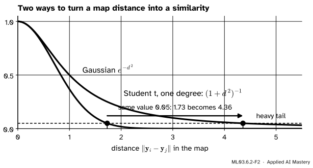
The two kernels agree near 0, but the Student t falls off slowly. A pair that the Gaussian would place 1.73 apart for a similarity of 0.05 sits 4.36 apart under the Student t.
Step 5. Why the heavy tail. Around a point in ten dimensions there is far more room at a moderate distance than at a small one, and a flat map cannot copy that: there is not enough area near \(i\) to hold all its moderately distant points. This is the crowding problem. With a Gaussian in the map, those points pile up near the middle and squeeze the clusters together. The heavy tail lets a moderate distance in the data become a large distance in the map, and the clusters separate.
Step 6. Compare the two. The cost is the Kullback-Leibler divergence, introduced here only as far as we need it (M09.3 treats it in full):
It is never negative and is 0 only when \({Q = P}\). It is not symmetric: a pair with large \(p_{ij}\) but small \(q_{ij}\) (neighbours drawn far apart) costs a lot, while a pair with small \(p_{ij}\) and larger \(q_{ij}\) costs little. So the cost cares most about keeping neighbours together.
The formal statement
NoteResult: the t-SNE gradient (van der Maaten and Hinton, equation 5)
Derivation. Write \({d_{ij} = \norm{\vect{y}_i - \vect{y}_j}^2}\), so that \({w_{ij} = (1 + d_{ij})^{-1}}\), and \({Z = \sum_{k \ne l} w_{kl}}\), so \({q_{ij} = w_{ij}/Z}\). Split the logarithm, and use \({\sum_{k \ne l} p_{kl} = 1}\) in the last term:
The second uses \({dw/dd = -(1 + d)^{-2} = -w^2}\). Only the pairs \((i, j)\) and \((j, i)\) involve \(\vect{y}_i\), and they are equal, so each sum over pairs picks up a factor 2:
Since \({w_{ij}/Z = q_{ij}}\), adding the two lines gives \({4\sum_j (p_{ij} - q_{ij})\,w_{ij}(\vect{y}_i - \vect{y}_j)}\), the result.
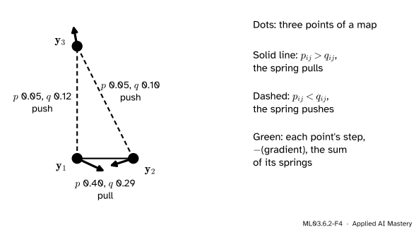
Read it as springs. Each other point \(j\) acts on \(\vect{y}_i\) along the line between them. A gradient step moves \(\vect{y}_i\) by \(-\eta\) times the gradient, so when \({p_{ij} > q_{ij}}\) (the map has them too far apart) the step pulls \(\vect{y}_i\) towards \(\vect{y}_j\), and when \({p_{ij} < q_{ij}}\) it pushes them apart. The factor \({w_{ij} = (1 + d_{ij})^{-1}}\) weakens the spring for pairs far apart in the map, but only like one over the distance squared, so distant clusters still feel each other.
ML03.6.2-F4
Three map points as springs. \(\vect{y}_1\) and \(\vect{y}_2\) should be closer (\({p > q}\)), so their spring pulls; the other two pairs are too close (\({p < q}\)) and push. Each green arrow, the sum of a point’s springs, is the step that the negative gradient prescribes (drawn 2.2 times longer to be seen).
Go deeper: symmetric SNE, and what the Student t changes
Put a Gaussian in the map instead, \({w_{ij} = e^{-d_{ij}}}\). Then \({\partial\log w_{ij}/\partial\vect{y}_i = -2(\vect{y}_i - \vect{y}_j)}\) and \({\partial w_{ij}/\partial\vect{y}_i = -2w_{ij}(\vect{y}_i - \vect{y}_j)}\), and the same two steps give \({4\sum_j(p_{ij} - q_{ij})(\vect{y}_i - \vect{y}_j)}\): the gradient of symmetric SNE in the paper’s Section 3.1. The springs are the same except for the factor \(w_{ij}\). With the Gaussian, a pair with \(p_{ij}\) a little above \(q_{ij}\) pulls harder the further apart it is, so the many moderately distant pairs drag everything to the middle. With the Student t that pull fades with distance.
Worked example
The neighbour probabilities of one of ten points. The ten points are two plus signs: \((0, 0)\), \((1, 0)\), \((0, 1)\), \((-1, 0)\), \((0, -1)\), and the same five shifted by \((4, 3)\). Take \({i = (1, 0)}\).
Distances. To its own group: 1 to \((0, 0)\), \({\sqrt2 = 1.414}\) to \((0, 1)\) and \((0, -1)\), and 2 to \((-1, 0)\). To the far group: from 3.61 to 5.
Weights with \({\sigma_i = 1}\).\({e^{-d^2/2}}\) gives \({e^{-0.5} = 0.6065}\), \({e^{-1} = 0.3679}\) twice and \({e^{-2} = 0.1353}\); the far five add only 0.0031. The total is 1.4808, so
So with \({\sigma_i = 1}\), \(i\) has about 3.6 effective neighbours: four in its group, one of them weaker.
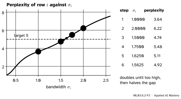
Search for a perplexity of 5. 3.64 is too low, so double \(\sigma_i\) to 2, which gives 6.22: too high. Halve the gap each time: 1.5 gives 4.74, 1.75 gives 5.48, 1.625 gives 5.11, 1.5625 gives 4.92. After 19 steps the search stops at \({\sigma_i = 1.589}\).
ML03.6.2-F3
Binary search for \(\sigma_i\). The perplexity rises steadily with \(\sigma_i\), so doubling until it is too high and then halving the gap closes in on the target of 5.
One symmetric probability. With every point at perplexity 5, the point \((0, 0)\) picks \((1, 0)\) with \({p_{j|i} = 0.235}\) and \((1, 0)\) picks \((0, 0)\) with 0.292, so
sigma = 1: [0.41  0.248 0.091 0.248]  H = 1.863  perplexity = 3.64
perplexity 5 needs sigma = 1.589 after 19 steps
p_ij for (0, 0), (1, 0): 0.0263   sum of P: 1.0   inside the groups: 0.937
Now the map side and the gradient. A derived gradient is only trusted once it agrees with finite differences: nudge one coordinate by a tiny amount and watch the cost change.
def q_probs(Y): w =1/ (1+ ((Y[:, None, :] - Y[None, :, :]) **2).sum(-1)) np.fill_diagonal(w, 0)return w / w.sum(), wdef kl(P, Q): m = P >0return (P[m] * np.log(P[m] / Q[m])).sum()def gradient(P, Y): Q, w = q_probs(Y) M = (P - Q) * w # (p_ij - q_ij) / (1 + d_ij)return4* (M.sum(axis=1)[:, None] * Y - M @ Y) # 4 sum_j M_ij (y_i - y_j)Y = np.random.default_rng(0).normal(size=(10, 2))g = gradient(P, Y)h, numeric =1e-6, np.zeros_like(Y)for i inrange(10):for a inrange(2): E = np.zeros_like(Y) E[i, a] = h numeric[i, a] = (kl(P, q_probs(Y + E)[0]) - kl(P, q_probs(Y - E)[0])) / (2* h)print("largest gap, formula against finite differences:", f"{np.abs(g - numeric).max():.1e}")Y3 = np.array([[0, 0], [1, 0], [0, 2]], dtype=float)P3 = np.array([[0, 0.4, 0.05], [0.4, 0, 0.05], [0.05, 0.05, 0]])Q3 = q_probs(Y3)[0]print("three map points: q_12, q_13, q_23 =", np.round([Q3[0, 1], Q3[0, 2], Q3[1, 2]], 4))
largest gap, formula against finite differences: 2.2e-10
three map points: q_12, q_13, q_23 = [0.2885 0.1154 0.0962]
The forces add up to zero over all points, as equal and opposite springs must. scikit-learn’s TSNE computes the same affinities and gradient; the next lesson runs it.
Explore
This module’s interactive, live t-SNE, lives in lesson 3. Set the perplexity to 2 and then to 50 on the “two clusters” preset and watch each point’s neighbourhood widen.
Pitfalls
ML03.6.2-F5
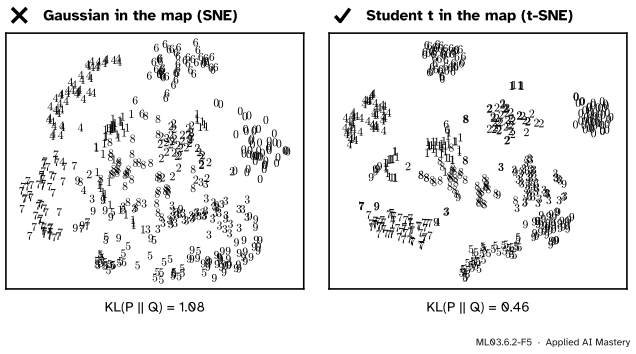
Wrong beside right, on the same affinities of 500 digits. With a Gaussian in the map, the digit groups crowd into one ball. With the Student t they become islands, and the map matches \(P\) far better.
“A Gaussian in the map is the natural choice, since the data use one.”
The data live in 64 dimensions and the map in 2, so the same curve cannot serve both: that is the crowding problem. The Student t is chosen because its tail is heavy, not because the data follow it. On 500 digits, symmetric SNE ends with \({\mathrm{KL} \approx 1.1}\) and no gaps; t-SNE on the same \(P\) ends near 0.46 with clear islands.
“The perplexity is the number of clusters (or of points per cluster).”
It is an effective number of neighbours per point. It sets each \(\sigma_i\) and so the scale of the neighbourhoods; it says nothing about how many groups there are. The next lesson shows the same data at perplexities from 2 to 100.
“A small KL means the whole layout is faithful.”
KL punishes neighbours drawn far apart, and barely punishes far points drawn near. A low cost certifies the neighbourhoods, not the distances between clusters.
Check yourself
Recall
1. What is \(p_{j|i}\), in words?
Show answer
The probability that point \(i\) would pick \(j\) as its neighbour if it chose in proportion to a Gaussian of width \(\sigma_i\) centred on itself.
2. How is the perplexity of a row defined, and what does it measure?
Show answer
\({2^{H_i}}\) with \({H_i = -\sum_j p_{j|i}\log_2 p_{j|i}}\). It is an effective number of neighbours.
3. How is the symmetric \(p_{ij}\) made from the conditional ones?
Show answer
\({p_{ij} = (p_{j|i} + p_{i|j})/2n}\).
4. Why does t-SNE use a Student t with one degree of freedom in the map?
Show answer
Its heavy tail lets moderate distances in the data become large distances in the map, which solves the crowding problem and lets clusters separate.
and the perplexity is \({2^{1.370} = 2.58}\): between two and three effective neighbours.
2.★★ Three map points sit at \({\vect{y}_1 = (0, 0)}\), \({\vect{y}_2 = (1, 0)}\) and \({\vect{y}_3 = (0, 2)}\). Compute \(q_{12}\), \(q_{13}\) and \(q_{23}\).
Show solution
The squared distances are 1, 4 and 5, so the kernel values are \({\tfrac12}\), \({\tfrac15}\) and \({\tfrac16}\). Each pair appears twice in the denominator: \({Z = 2(\tfrac12 + \tfrac15 + \tfrac16) = 1.7333}\). Then \({q_{12} = 0.5/1.7333 = 0.2885}\), \({q_{13} = 0.2/1.7333 = 0.1154}\) and \({q_{23} = 0.1667/1.7333 = 0.0962}\); twice their sum is 1.
3.★★★ Show that the gradient pushes the map’s centre of mass nowhere: the gradients of all the points add up to the zero vector. What does this mean for the optimisation?
Show solution
Write \({\vect{f}_{ij} = 4(p_{ij} - q_{ij})w_{ij}(\vect{y}_i - \vect{y}_j)}\), so the gradient at \(i\) is \({\sum_j \vect{f}_{ij}}\). Since \(p\), \(q\) and \(w\) are symmetric and \({\vect{y}_j - \vect{y}_i}\) is minus \({\vect{y}_i - \vect{y}_j}\), \({\vect{f}_{ji} = -\vect{f}_{ij}}\). Summing over all \(i\) and \(j\), each pair appears once each way and cancels, so \({\sum_i \partial C/\partial\vect{y}_i = \vect{0}}\). Every gradient step therefore leaves the mean of the map points where it was: the map does not drift, which is why it can start at the origin. The code above checks this numerically.
Summary card
Match neighbour probabilities, with a heavy tail in the map.
Sources. Each was opened and checked against this lesson on 15 November 2026.
Laurens van der Maaten and Geoffrey Hinton, Visualizing Data using t-SNE, Journal of Machine Learning Research 9 (2008), 2579–2605. Section 2 defines \(p_{j|i}\) (equation 1), the perplexity \({2^{H(P_i)}}\) with \(H\) in bits, the binary search for \(\sigma_i\), and typical perplexities between 5 and 50. Section 3.1 sets \({p_{ij} = (p_{j|i} + p_{i|j})/2n}\) and gives the symmetric SNE gradient; Section 3.2 describes the crowding problem; Section 3.3 gives the Student-t \(q_{ij}\) (equation 4) and the gradient (equation 5), derived in Appendix A.
scikit-learn 1.9 User Guide, Section 2.2.9, t-distributed Stochastic Neighbor Embedding. Describes Gaussian joint probabilities in the data and Student-t ones in the map, the KL divergence minimised by gradient descent, and the perplexity as \({2^S}\) with \(S\) the Shannon entropy.