Run PCA in the lifted space of a kernel without ever building it. Derive the centred Gram matrix, project training and new points with kernel sums, separate two rings that no line can, and see what the kernel width does, what it costs and why there is no way back.
ML03.5.4L2 Intermediate25 minIn review (what this means)
The maths and code on this page are checked by automated tests on every change, but an independent reader has not signed it off yet. Spot a mistake or a confusing step? Tell us.
Explain kernel PCA as the Gram-matrix route to PCA of ML03.5.2 with dot products replaced by a kernel.
Derive the centred Gram matrix K-tilde = K - 1_n K - K 1_n + 1_n K 1_n, and project training points and new points with it.
Carry out kernel PCA by hand for four values and a polynomial kernel, and with an RBF kernel and numpy.linalg.eigh on make_circles.
Match sklearn.decomposition.KernelPCA, and judge the effect of gamma, the n by n cost and the pre-image problem.
The question
Two rings of points, one inside the other. PCA projects onto straight lines, and no straight line can put one ring on one side and the other ring on the other side, so its components mix the rings. Yet the rings are obviously two groups. Can PCA be bent to follow curved structure, and what does that cost?
From the last lesson
1. What is the covariance of \(\vect{x}\) under probabilistic PCA?
Show answer
\({\mat{W}\mat{W}\T + \sigma^2\mat{I}}\).
2. How is the number of components chosen with that model?
Show answer
By the held-out log-likelihood, for example cross_val_score with PCA.score.
Intuition
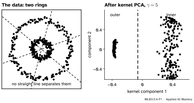
ML02.8 lifted data into a bigger space where a straight line works. Kernel PCA does the same for PCA: lift every point, run PCA up there, and read off the scores. Here is the result on the two rings.
ML03.5.4-F1
Kernel PCA with an RBF kernel. In the plane the rings cannot be split by a line; along the first kernel component they fall apart, and one cut separates them.
The lift is never written down. ML03.5.2 showed that PCA’s scores can be found from the dot products of the points alone, through the \({n \times n}\) matrix \({\mat{X}_c\mat{X}_c\T}\). A kernel\({k(\vect{x}, \vect{z})}\) is a dot product in a lifted space, \({\phi(\vect{x}) \cdot \phi(\vect{z})}\), computed without building \(\phi\) (ML02.8). Put the two together and PCA runs in the lifted space at the cost of an \({n \times n}\) eigenproblem.
Build it up
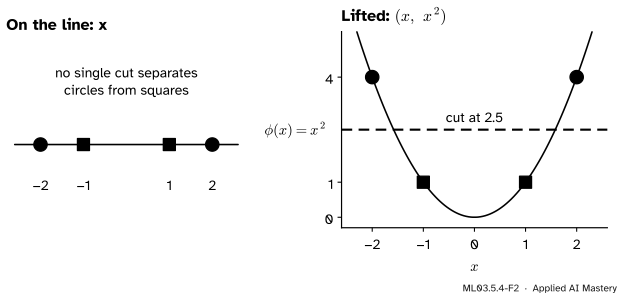
Step 1. A lift you can see. Take four values on a line, \({x = -2, -1, 1, 2}\), with \(\pm 1\) in one group and \(\pm 2\) in the other. No single cut on the line separates them. Lift each value to \({(x, x^2)}\) and they can be cut at height 2.5.
ML03.5.4-F2
A one-dimensional picture of the rings. The lift \({\phi(x) = x^2}\) puts the two groups at different heights.
Step 2. The kernel trick, in one paragraph. For this lift, \({\phi(x)\phi(z) = x^2z^2}\), so the kernel is \({k(x, z) = x^2z^2}\). Most kernels hide a lift too big to write: the RBF kernel \({k(\vect{x}, \vect{z}) = \exp(-\gamma\norm{\vect{x} - \vect{z}}^2)}\) is a dot product in an infinite-dimensional space. All we ever use is the Gram matrix\(\mat{K}\), with \({K_{ij} = k(\vect{x}_i, \vect{x}_j)}\).
Step 3. Centre in the lifted space. PCA needs centred points, \({\tilde{\phi}_i = \phi(\vect{x}_i) - \bar{\phi}}\) with \({\bar{\phi} = \tfrac1n\sum_l \phi(\vect{x}_l)}\). We cannot subtract \(\bar{\phi}\) directly, but we can find every dot product of centred points from \(\mat{K}\), as the next section shows.
Step 4. Eigen-decompose and read off scores. With the centred Gram matrix \(\tilde{\mat{K}}\) in hand, ML03.5.2’s recipe applies unchanged: an eigenpair \({\tilde{\mat{K}}\vect{a} = \mu\vect{a}}\) with unit \(\vect{a}\) gives the scores \({\sqrt{\mu}\,\vect{a}}\) of the training points on that component.
The formal statement
Centring the Gram matrix. Expand the dot product of two centred lifted points:
Each term is a kernel value or an average of kernel values. Let \(\mat{1}_n\) be the \({n \times n}\) matrix with every entry \({1/n}\). Then \({\mat{1}_n\mat{K}}\) holds the column means and \({\mat{K}\mat{1}_n}\) the row means, so
Since \({\mat{J} = \mat{I} - \mat{1}_n}\), this is \({\mat{J}\mat{K}\mat{J}}\): the same double centring that turned distances into dot products in ML03.5.2.
Projecting. By ML03.5.2, the unit direction of component \(j\) in the lifted space is \({\vect{v}_j = \sum_i a_{ij}\tilde{\phi}_i/\sqrt{\mu_j}}\). The score of any point \(\vect{x}\) is \({\tilde{\phi}(\vect{x}) \cdot \vect{v}_j}\), a sum of centred kernel values:
For a training point \({\vect{x} = \vect{x}_i}\), \(\tilde{\vect{k}}\) is row \(i\) of \(\tilde{\mat{K}}\), and the score is \({(\tilde{\mat{K}}\vect{a}_j)_i/\sqrt{\mu_j} = \sqrt{\mu_j}\,a_{ij}}\), as in Step 4.
ML03.5.4-F5
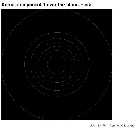
The first kernel component is a function on the whole plane, a sum of RBF bumps, one per training point. Projecting a new point is reading this landscape at its position.
What \(\gamma\) does. For small \(\gamma\), \({e^{-\gamma s} \approx 1 - \gamma s}\), so \({K_{ij} \approx 1 - \gamma\norm{\vect{x}_i - \vect{x}_j}^2}\). Double centring removes the constant and, as in ML03.5.2, turns \({-\norm{\vect{x}_i - \vect{x}_j}^2}\) into \({2\,\vect{c}_i \cdot \vect{c}_j}\): \({\tilde{\mat{K}} \approx 2\gamma\,\mat{X}_c\mat{X}_c\T}\), and kernel PCA becomes plain PCA. For large \(\gamma\), every bump is so narrow that \({\mat{K} \approx \mat{I}}\): each point is alone, all eigenvalues are alike, and the components pick out a few points at random. The useful \(\gamma\) lies between, at the scale of the gaps in the data.
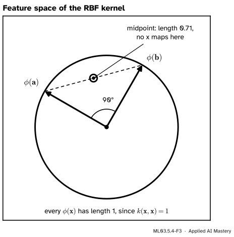
The pre-image problem. A score lives in the lifted space, and some points there are the image of no data point. For the RBF kernel \({\norm{\phi(\vect{x})}^2 = k(\vect{x}, \vect{x}) = 1}\): every image lies on a sphere of radius 1.
ML03.5.4-F3
Images of points under the RBF kernel lie on the unit sphere. The average of two images lies inside it, so no point of the data space maps there.
The midpoint of \({\phi(\vect{a})}\) and \({\phi(\vect{b})}\) has squared length
which is less than 1 whenever \({\vect{a} \ne \vect{b}}\). So “go back to the data space”, which was \({\bar{\vect{x}} + \mat{Q}_q\vect{y}}\) for PCA, has no exact answer here. scikit-learn’s fit_inverse_transform=True learns an approximate way back by kernel ridge regression from scores to points (Bakır, Weston and Schölkopf).
Worked example
Four values, \({k(x, z) = x^2z^2}\). Kernel PCA by hand, then a check against the lift \({\phi(x) = x^2}\), which we can see.
ML03.5.4-F4
Kernel PCA of four values by hand. The kernel component reproduces the centred lift exactly.
Gram matrix. With \({x^2 = (4, 1, 1, 4)}\), \({K_{ij}}\) is the product of the squares: the first row is \({(16, 4, 4, 16)}\), the second \({(4, 1, 1, 4)}\). The row means are 10, 2.5, 2.5 and 10, and the overall mean is 6.25.
Centre.\({\tilde{K}_{11} = 16 - 10 - 10 + 6.25 = 2.25}\) and \({\tilde{K}_{12} = 4 - 10 - 2.5 + 6.25 = -2.25}\). Every entry is \(\pm 2.25\): \({\tilde{\mat{K}} = 2.25\,\vect{s}\vect{s}\T}\) with \({\vect{s} = (1, -1, -1, 1)}\).
Eigen. A matrix \({2.25\,\vect{s}\vect{s}\T}\) has one nonzero eigenvalue, \({2.25 \times \norm{\vect{s}}^2 = 9}\), with unit eigenvector \({\vect{a} = \vect{s}/2}\).
Project. The scores are \({\sqrt{9}\,\vect{a} = (1.5, -1.5, -1.5, 1.5)}\). Check with the lift: \({\phi = (4, 1, 1, 4)}\) has mean 2.5, so the centred lift is exactly \({(1.5, -1.5, -1.5, 1.5)}\). The groups sit at \(+1.5\) and \(-1.5\), separated as in the figure of Step 1.
A new value\({x = 0}\). All \({k(x_i, 0) = 0}\), so \({\tilde{k}_i = 0 - 0 - r_i + 6.25}\), which is \({(-3.75, 3.75, 3.75, -3.75)}\). Its score is \({\tilde{\vect{k}} \cdot \vect{a}/3 = -7.5/3 = -2.5}\), and indeed \({\phi(0) - 2.5 = -2.5}\).
Code
The worked example first, then the rings with the RBF kernel and numpy.linalg.eigh.
import numpy as npdef centre_gram(K): n =len(K) one = np.full((n, n), 1/ n)return K - one @ K - K @ one + one @ K @ onex = np.array([-2.0, -1.0, 1.0, 2.0])K = np.outer(x **2, x **2)Kt = centre_gram(K)mu, A = np.linalg.eigh(Kt)mu, a = mu[-1], A[:, -1] * np.sign(A[0, -1])print("centred Gram:\n", Kt)print("eigenvalue:", round(mu, 6), " scores:", (np.sqrt(mu) * a).round(6))k_new = np.zeros(4) # k(x_i, 0) = 0 for every ikt_new = k_new - k_new.mean() - K.mean(axis=1) + K.mean()print("score of x = 0:", round(kt_new @ a / np.sqrt(mu), 6))
from sklearn.datasets import make_circlesfrom sklearn.decomposition import PCA, KernelPCAX, ring = make_circles(n_samples=400, factor=0.3, noise=0.05, random_state=0) # ring 1 is the inner onedef rbf(A, B, gamma): d2 = (A **2).sum(1)[:, None] + (B **2).sum(1)[None, :] -2* A @ B.Treturn np.exp(-gamma * np.maximum(d2, 0))gamma =5.0K = rbf(X, X, gamma)mu, A = np.linalg.eigh(centre_gram(K))mu, A = mu[::-1], A[:, ::-1]A = A * np.sign(A[np.abs(A).argmax(axis=0), range(len(A))]) # fix each component's signscores = A[:, :2] * np.sqrt(mu[:2])print("inner ring on component 1:", scores[ring ==1, 0].min().round(3), "to", scores[ring ==1, 0].max().round(3))print("outer ring on component 1:", scores[ring ==0, 0].min().round(3), "to", scores[ring ==0, 0].max().round(3))lib = KernelPCA(n_components=2, kernel="rbf", gamma=gamma).fit(X)print("library agrees up to signs:", np.allclose(np.abs(lib.transform(X)), np.abs(scores), atol=1e-6)," eigenvalues:", lib.eigenvalues_.round(2))new = np.array([[0.0, 0.0], [1.0, 0.0]])k = rbf(new, X, gamma)kt = k - k.mean(axis=1, keepdims=True) - K.mean(axis=0)[None, :] + K.mean() # training averagesprint("new points on component 1:", (kt @ A[:, 0] / np.sqrt(mu[0])).round(3))
inner ring on component 1: 0.199 to 0.52
outer ring on component 1: -0.387 to -0.333
library agrees up to signs: True   eigenvalues: [56.8  41.39]
new points on component 1: [ 0.598 -0.379]
The inner ring lands between 0.20 and 0.52 on component 1, the outer between \(-0.39\) and \(-0.33\): a single cut separates them, which no line in the plane could do. A new point at the centre scores 0.60, with the inner ring; one at \((1, 0)\) scores \(-0.38\), with the outer.
Now \(\gamma\). For each value we ask how well the best single cut on component 1 separates the rings.
def best_cut(z, labels):returnmax(max(np.mean((z > c) == labels), np.mean((z < c) == labels)) for c in np.unique(z))for g in (0.1, 1.0, 5.0, 100.0): z = KernelPCA(n_components=1, kernel="rbf", gamma=g).fit_transform(X)[:, 0]print(f"gamma = {g:5}: best cut on component 1 is right for {best_cut(z, ring):.0%}")print(f"plain PCA: best cut on component 1 is right for {best_cut(PCA(1).fit_transform(X)[:, 0], ring):.0%}")print("linear kernel = PCA:", np.allclose(np.abs(KernelPCA(2, kernel="linear").fit_transform(X)), np.abs(PCA(2).fit_transform(X))))
gamma =   0.1: best cut on component 1 is right for 69%
gamma =   1.0: best cut on component 1 is right for 64%
gamma =   5.0: best cut on component 1 is right for 100%
gamma = 100.0: best cut on component 1 is right for 75%
plain PCA:     best cut on component 1 is right for 69%
linear kernel = PCA: True
Small \(\gamma\) behaves like plain PCA (69%, no better than PCA itself); \(\gamma = 5\) separates the rings perfectly; \(\gamma = 100\) falls apart. Last, the cost and the way back.
for n in (400, 10_000, 100_000):print(f"n = {n:>7,}: the Gram matrix alone takes {8* n * n /1e9:,.3f} GB")back = KernelPCA(n_components=2, kernel="rbf", gamma=gamma, fit_inverse_transform=True, alpha=0.1).fit(X)rebuilt = back.inverse_transform(back.transform(X))print("mean squared error of the learned way back:", round(np.mean(np.sum((X - rebuilt) **2, axis=1)), 3))a = X[ring ==0][:1] # a point of the outer ring, and the point opposite itprint("length of the midpoint of their images:", round(np.sqrt((1+ rbf(a, -a, gamma)[0, 0]) /2), 3))
n =     400: the Gram matrix alone takes 0.001 GB
n =  10,000: the Gram matrix alone takes 0.800 GB
n = 100,000: the Gram matrix alone takes 80.000 GB
mean squared error of the learned way back: 0.277
length of the midpoint of their images: 0.707
With two components the learned way back misses by 0.28 in squared distance on average, against squared distances of about 1 from the centre for the outer ring: the kernel components keep which ring, not where on the ring.
Explore
The module’s interactive, variance and error, is in lesson ML03.5.1. Load the round cloud and turn the line: every direction does about equally well, because in the plane the cloud has no long axis. That is the rings’ problem too, and kernel PCA solves it by lifting the points to a space where the inner and outer points differ along one direction.
Pitfalls
ML03.5.4-F6
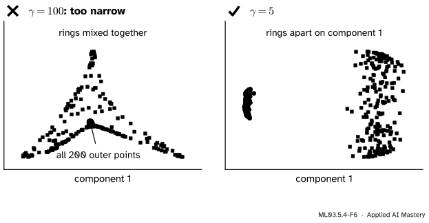
Wrong beside right. With \(\gamma = 100\) every bump is narrow: the leading components trace where a point sits around the dense inner ring, and the whole outer ring lands on one spot among them. With \(\gamma = 5\) the first component separates the rings.
“A larger \(\gamma\) is more flexible, so it is always at least as good.”
As \(\gamma\) grows, each bump narrows until only close neighbours still see each other; in the limit \({\mat{K} \to \mat{I}}\) and every point is an island of its own. Already at \(\gamma = 100\) the leading components follow fine detail, where a point sits around the dense inner ring, and squeeze the whole outer ring onto one spot in their middle, so the best cut on component 1 falls to 75%. As \(\gamma\) shrinks, kernel PCA turns into plain PCA. Choose \(\gamma\) at the scale of the data, by looking, or by validating whatever uses the components downstream.
“To project the test set, run kernel PCA on the test set.”
That fits new components with their own signs, order and centring, so test scores are not comparable with training scores. Project new points with the training points’ kernel values and the training averages, as transform does and as the formula above says.
“Kernel PCA scales like PCA.”
PCA solves a \({d \times d}\) eigenproblem; kernel PCA solves an \({n \times n}\) one, whatever \(d\) is. The Gram matrix has \(n^2\) entries, 1.28 MB for 400 points but 80 GB for 100,000, and a full eigendecomposition takes order \(n^3\) steps. For many points ask for few components with eigen_solver="randomized", or approximate the kernel with the Nyström method of ML02.8.4.
Check yourself
Recall
1. Which matrix does kernel PCA eigen-decompose?
Show answer
The centred Gram matrix \({\tilde{\mat{K}} = \mat{K} - \mat{1}_n\mat{K} - \mat{K}\mat{1}_n + \mat{1}_n\mat{K}\mat{1}_n}\), which is \({\mat{J}\mat{K}\mat{J}}\).
2. How are the training points’ scores read off an eigenpair \({(\mu, \vect{a})}\)?
Show answer
As \({\sqrt{\mu}\,\vect{a}}\), with \(\vect{a}\) of unit length.
3. What does a new point need in order to be projected?
Show answer
Its kernel values with every training point, centred with the training averages, then \({\tilde{\vect{k}} \cdot \vect{a}_j/\sqrt{\mu_j}}\) for component \(j\).
4. What does kernel PCA with an RBF kernel become when \(\gamma\) is very small, and when it is very large?
Show answer
Very small: plain PCA, since \({\tilde{\mat{K}} \approx 2\gamma\mat{X}_c\mat{X}_c\T}\). Very large: \({\mat{K} \approx \mat{I}}\), every point alone, and the components show no structure.
5. Why can kernel PCA not decode exactly?
Show answer
Some points of the lifted space are the image of no data point; for the RBF kernel every image has length 1, and averages of images are shorter. inverse_transform only learns an approximation.
Exercises
1.★ Show that with the linear kernel \({k(\vect{x}, \vect{z}) = \vect{x} \cdot \vect{z}}\), the centred Gram matrix is \({\mat{X}_c\mat{X}_c\T}\), so kernel PCA is PCA.
Show solution
Here \({\mat{K} = \mat{X}\mat{X}\T}\), so \({\tilde{\mat{K}} = \mat{J}\mat{X}\mat{X}\T\mat{J} = (\mat{J}\mat{X})(\mat{J}\mat{X})\T}\). And \({\mat{J}\mat{X} = \mat{X}_c}\), because \(\mat{J}\) subtracts the column means. By ML03.5.2 its eigenpairs give the PCA scores.
2.★★ For the four values with \({k(x, z) = x^2z^2}\), project \({x = 3}\).
Show solution
\({k(x_i, 3) = 9x_i^2 = (36, 9, 9, 36)}\), with mean 22.5. So \({\tilde{k}_i = k(x_i, 3) - 22.5 - r_i + 6.25}\), which is \({36 - 22.5 - 10 + 6.25 = 9.75}\) for \({x_i = \pm 2}\) and \({9 - 22.5 - 2.5 + 6.25 = -9.75}\) for \({x_i = \pm 1}\). The score is \({\tilde{\vect{k}} \cdot \vect{a}/3 = (4 \times 9.75 \times \tfrac12)/3 = 6.5}\), and indeed \({\phi(3) - 2.5 = 9 - 2.5 = 6.5}\).
3.★★★ Show that for the RBF kernel the midpoint \({\tfrac12(\phi(\vect{a}) + \phi(\vect{b}))}\) of two different points has no pre-image: no \(\vect{x}\) has \(\phi(\vect{x})\) equal to it.
Show solution
Every image has squared length \({k(\vect{x}, \vect{x}) = e^0 = 1}\). The midpoint has squared length
For \({\vect{a} \ne \vect{b}}\), \({k(\vect{a}, \vect{b}) = e^{-\gamma\norm{\vect{a} - \vect{b}}^2} < 1}\), so the squared length is below 1, and no image can equal it.
Summary card
Kernel PCA is PCA by the Gram route, with dot products replaced by a kernel.
ML03.5.4-F1
Lift, centre, eigen-decompose.
Centre.\({\tilde{\mat{K}} = \mat{J}\mat{K}\mat{J}}\), with \({\mat{J} = \mat{I} - \mat{1}_n}\).
Training scores.\({\sqrt{\mu_j}\,\vect{a}_j}\) from \({\tilde{\mat{K}}\vect{a}_j = \mu_j\vect{a}_j}\).
New points.\({\tilde{\vect{k}}(\vect{x}) \cdot \vect{a}_j/\sqrt{\mu_j}}\), centred with training averages.
Watch.\(\gamma\), the \({n \times n}\) cost, and no exact way back.
Sources and next steps
Sources. Each was opened and checked against this lesson on 15 November 2026.
Bernhard Schölkopf, Alexander Smola and Klaus-Robert Müller, Nonlinear component analysis as a kernel eigenvalue problem, Max Planck Institute for Biological Cybernetics, Technical Report 44 (December 1996), the report behind the paper in Neural Computation 10 (1998). The eigenproblem (12), the normalisation (16), projections of test points as kernel sums (24), and in Appendix A the centred kernel matrix (49) and its version for test points (54).
Christopher M. Bishop, Pattern Recognition and Machine Learning, Section 12.3: equations (12.84) and (12.85) centre the Gram matrix, and a linear kernel recovers standard PCA.
Trevor Hastie, Robert Tibshirani and Jerome Friedman, The Elements of Statistical Learning, Section 14.5.4: kernel PCA as the eigen-decomposition of the double-centred Gram matrix \({(\mat{I} - \mat{M})\mat{K}(\mat{I} - \mat{M})}\) (14.65), mimicking PCA from the inner-product matrix.
scikit-learn 1.9, sklearn.decomposition.KernelPCA (eigenvalues_ are those of the centred kernel matrix; fit_inverse_transform learns pre-images following Bakır, Weston and Schölkopf, NIPS 16, 2004), the example Kernel PCA on make_circles, and the User Guide, Section 2.5.2: inverse_transform relies on kernel ridge regression and is an approximation, and the exact method costs order \({n^3}\).
Next. ML03.6, manifold learning, follows curved structure with neighbourhood graphs instead of a kernel, and reuses classical MDS from ML03.5.2 for Isomap.