Give PCA a story: a few hidden numbers, a linear map and round noise. Its maximum-likelihood fit has a closed form built from the eigenvectors, its likelihood chooses the number of components on held-out data, and factor analysis lets each feature keep its own noise.
ML03.5.3L2 Intermediate25 minIn review (what this means)
The maths and code on this page are checked by automated tests on every change, but an independent reader has not signed it off yet. Spot a mistake or a confusing step? Tell us.
State the probabilistic PCA model x = W z + mu + noise and derive that x has covariance W W-transpose + sigma^2 I.
Compute the closed-form maximum-likelihood fit of Tipping and Bishop, with sigma^2 the mean of the discarded eigenvalues, and check numerically that it is a maximum.
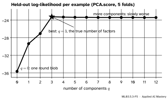
Choose the number of components by the held-out log-likelihood of PCA.score.
Explain how factor analysis differs, fit it with sklearn.decomposition.FactorAnalysis, and recognise data where it beats probabilistic PCA.
The question
PCA so far is geometry: directions, projections, errors. It assigns no probability to anything, so it cannot say how surprising a new point is, and it cannot compare \(q = 3\) with \(q = 4\) except by a rule of thumb. Is there a probability model whose best fit is PCA, and what does it give us that plain PCA cannot?
From the last lesson
1. What two moves make up PCA whitening?
Show answer
Rotate onto the principal axes with \(\mat{Q}\T\), then divide each coordinate by \(\sqrt{\lambda_j}\).
2. What does double centring a matrix of squared distances give?
Show answer
\({-\tfrac12\mat{J}\mat{D}^{(2)}\mat{J} = \mat{X}_c\mat{X}_c\T}\), the dot products of the centred points.
Intuition
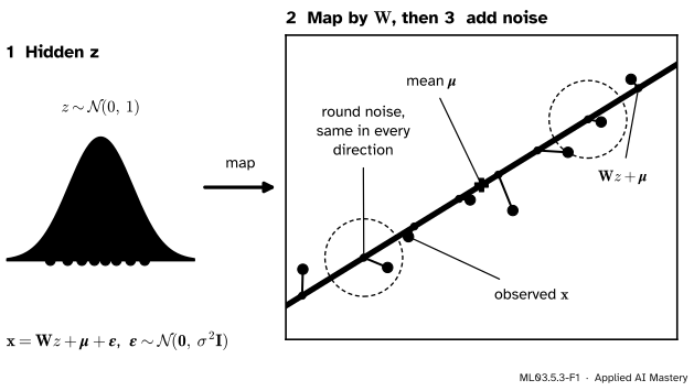
Tell a story of how the data were made. First draw a few hidden numbers, the latent variables\(\vect{z}\). Then map them linearly into the data space and shift by a mean. Last, blur every point with a little noise that is the same in every direction.
ML03.5.3-F1
The story of probabilistic PCA for the four points, with one hidden number. A standard normal \(z\) picks a place on the orange line; round noise moves the point off it.
This is probabilistic PCA (PPCA), introduced by Tipping and Bishop. With one latent variable the data lie near a line; with \(q\) of them, near a flat of dimension \(q\). The flat is where the structure lives and the noise is what PCA throws away. The surprise is that the best-fitting line of this story is exactly the first principal direction, so we keep everything PCA gave us and gain a likelihood.
Build it up
Step 1. The model. For each example, independently,
with \(\vect{z}\) and \(\vect{\epsilon}\) independent. The parameters are the \({d \times q}\) matrix \(\mat{W}\) of loadings, the mean \(\vect{\mu}\) and the noise variance \(\sigma^2\).
Step 2. The distribution of \(\vect{x}\). A linear map of Gaussians plus a Gaussian is Gaussian (M07.3 proves this), so we need only its mean and covariance. The mean is \(\vect{\mu}\), since \(\vect{z}\) and \(\vect{\epsilon}\) have mean zero. For the covariance, expand:
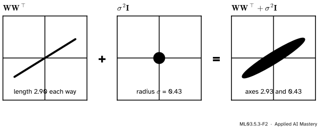
The cross terms \({\mat{W}\E[\vect{z}\vect{\epsilon}\T]}\) and its transpose vanish because \(\vect{z}\) and \(\vect{\epsilon}\) are independent with mean zero. So \({\vect{x} \sim \mathcal{N}(\vect{\mu}, \mat{\Sigma})}\) with \({\mat{\Sigma} = \mat{W}\mat{W}\T + \sigma^2\mat{I}}\).
ML03.5.3-F2
The model’s covariance for the four points with \(q = 1\): a flat ellipse along \(\mat{W}\) plus a round one of radius \(\sigma\). Along \(\mat{W}\) the spreads add; across it only the noise is left.
Step 3. The likelihood. For a data set, the log-likelihood (S02.3) is the sum of the log densities. With \(\vect{\mu}\) at the sample mean it can be written with the maximum-likelihood covariance\({\mat{S} = \tfrac1n\sum_i (\vect{x}_i - \bar{\vect{x}})(\vect{x}_i - \bar{\vect{x}})\T}\), which divides by \(n\):
The trace appears because each quadratic form \({(\vect{x}_i - \bar{\vect{x}})\T\mat{\Sigma}^{-1}(\vect{x}_i - \bar{\vect{x}})}\) is a \({1 \times 1}\) matrix, equal to its own trace, and \({\operatorname{tr}(\vect{a}\T\mat{M}\vect{a}) = \operatorname{tr}(\mat{M}\vect{a}\vect{a}\T)}\); summing over \(i\) gives \({n\operatorname{tr}(\mat{\Sigma}^{-1}\mat{S})}\).
The formal statement
NoteThe maximum-likelihood fit (Tipping and Bishop)
Let \(\mat{S}\) have eigenvalues \({\lambda_1 \ge \cdots \ge \lambda_d}\) with orthonormal eigenvectors \({\vect{u}_1, \dots, \vect{u}_d}\), and let \(\mat{U}_q\) hold the first \(q\) of them. The log-likelihood is largest at \({\vect{\mu} = \bar{\vect{x}}}\),
where \({\mat{\Lambda}_q}\) holds \({\lambda_1, \dots, \lambda_q}\) and \(\mat{R}\) is any \({q \times q}\) orthogonal matrix.
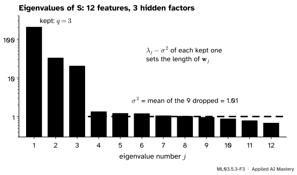
So the loadings point along the principal directions, the noise is the average variance PCA throws away, and column \(j\) of \(\mat{W}\) (with \({\mat{R} = \mat{I}}\)) has length \({\sqrt{\lambda_j - \sigma^2}}\). \(\mat{R}\) is free because \({\mat{W}\mat{R}\mat{R}\T\mat{W}\T = \mat{W}\mat{W}\T}\): turning the hidden space changes nothing we can observe.
ML03.5.3-F3
The fit read off the spectrum. The kept eigenvalues stand far above a floor of nearly equal small ones; \(\sigma^2\) is the height of that floor, here 1.01 against a true noise variance of 1.
What the fitted model looks like. With \({\mat{R} = \mat{I}}\), \({\mat{W}\mat{W}\T = \mat{U}_q(\mat{\Lambda}_q - \sigma^2\mat{I})\mat{U}_q\T}\). Add \(\sigma^2\mat{I}\) and look along each eigenvector: along \(\vect{u}_j\) with \({j \le q}\) the variance is \({(\lambda_j - \sigma^2) + \sigma^2 = \lambda_j}\), the data’s own; along every other \(\vect{u}_j\) it is \(\sigma^2\). So the model copies the data’s spread in the \(q\) principal directions and replaces the rest by one average.
Why the average. Hold the kept part of the model fixed, with variance \(\lambda_j\) along each \(\vect{u}_j\) for \({j \le q}\), and let only the variance \(\sigma^2\) of the other \({d - q}\) directions vary. Those directions contribute \({(d - q)\ln\sigma^2}\) to \(\ln\det\mat{\Sigma}\) and \({\sum_{j>q}\lambda_j/\sigma^2}\) to the trace; the kept directions add terms that do not depend on \(\sigma^2\). Writing \(s\) for \(\sigma^2\), we minimise \({f(s) = (d - q)\ln s + \tfrac{1}{s}\sum_{j>q}\lambda_j}\):
Since \({f'(s)}\) is negative below this value and positive above it, it is the minimum.
That \(\mat{W}\) must lie along the top eigenvectors is Tipping and Bishop’s harder result: every other choice of eigenvectors is a saddle point of the likelihood. The code checks numerically that 300 random small changes of the fitted parameters all lower the likelihood.
The maximum value. With these parameters, \({\ln\det\mat{\Sigma} = \sum_{j \le q}\ln\lambda_j + (d - q)\ln\sigma^2}\) and \({\operatorname{tr}(\mat{\Sigma}^{-1}\mat{S}) = q + (d - q) = d}\), so
The codes. Given \(\vect{x}\), the hidden \(\vect{z}\) is uncertain, and Bayes’ rule gives its mean: \({\E[\vect{z} \mid \vect{x}] = \mat{M}^{-1}\mat{W}\T(\vect{x} - \vect{\mu})}\) with \({\mat{M} = \mat{W}\T\mat{W} + \sigma^2\mat{I}}\). For one component \({\mat{M} = \lambda_1}\), and the code is the PCA score multiplied by \({\sqrt{\lambda_1 - \sigma^2}/\lambda_1}\). That is the whitened score (ML03.5.2, here dividing by \(\sqrt{\lambda_1}\) of \(\mat{S}\)) times \({\sqrt{1 - \sigma^2/\lambda_1}}\): pulled slightly towards zero, more so the noisier the data.
Factor analysis keeps the story but gives each feature its own noise: \({\vect{\epsilon} \sim \mathcal{N}(\vect{0}, \mat{\Psi})}\) with \(\mat{\Psi}\) diagonal, so \({\mat{\Sigma} = \mat{W}\mat{W}\T + \mat{\Psi}}\). There is no closed form; it is fitted iteratively. In exchange, a feature that is simply measured badly can be explained by its own large \(\psi_j\) instead of bending \(\mat{W}\) towards it.
Worked example
The four points, \(q = 1\). Dividing the scatter matrix by \(n = 4\),
Probabilistic PCA of the four points by the closed form.
Eigenvalues. They are a quarter of the scatter matrix’s, \({(35 \pm 15\sqrt5)/8}\), so \({\lambda_1 \approx 8.568}\) and \({\lambda_2 \approx 0.182}\), with the same eigenvector \({\vect{u}_1 \approx (0.851, 0.526)}\) as in M03.6.
Noise. One eigenvalue is dropped, so \({\sigma^2 = \lambda_2 \approx 0.182}\).
Loadings.\({\sqrt{8.568 - 0.182} \approx 2.896}\), so \({\mat{W} \approx (2.463, 1.522)}\), a column.
Check.\({\mat{W}\mat{W}\T + \sigma^2\mat{I}}\) has variance \({8.386 + 0.182 = 8.568}\) along \(\vect{u}_1\) and \(0.182\) across it, the eigenvalues of \(\mat{S}\), so it is\(\mat{S}\). With \({d - q = 1}\) nothing is averaged and the fit is exact. The log-likelihood is
Codes. The PCA score of \((0, 1)\) is \(-4.03\); the code is \({-4.03 \times 2.896 / 8.568} \approx -1.36\), slightly less than the whitened score \({-4.03/\sqrt{8.568}} \approx -1.38\).
Code
The closed form, from scratch, and the log-likelihood both ways.
import numpy as npdef ppca(X, q):"""Maximum-likelihood probabilistic PCA (Tipping and Bishop): mean, W, sigma^2, eigenvalues of S.""" m = X.mean(axis=0) S = (X - m).T @ (X - m) /len(X) # divides by n lam, U = np.linalg.eigh(S) lam, U = lam[::-1], U[:, ::-1] U = U * np.sign(U[np.abs(U).argmax(axis=0), range(U.shape[1])]) # fix each sign s2 = lam[q:].mean()return m, U[:, :q] * np.sqrt(lam[:q] - s2), s2, lamdef loglik(X, m, Sigma): n, d = X.shape Xc = X - m quad = np.einsum("ij,jk,ik->", Xc, np.linalg.inv(Sigma), Xc)return-0.5* n * (d * np.log(2* np.pi) + np.linalg.slogdet(Sigma)[1]) -0.5* quadP = np.array([[0.0, 1.0], [3.0, 2.0], [4.0, 4.0], [7.0, 5.0]])m, W, s2, lam = ppca(P, 1)Sigma = W @ W.T + s2 * np.eye(2)print("eigenvalues of S:", lam.round(3), " sigma^2:", round(s2, 3), " W:", W.ravel().round(3))print("model covariance:\n", Sigma.round(4))print("log-likelihood:", round(loglik(P, m, Sigma), 2))print("codes E[z | x]:", ((P - m) @ W / (W.T @ W + s2)).ravel().round(2))
The four points are too few to test the claim that this is a maximum. Make 200 examples of 12 features from 3 hidden factors with noise variance 1, fit \(q = 3\), and nudge the parameters at random: every nudge lowers the likelihood.
rng = np.random.default_rng(3)W_true = rng.normal(size=(12, 3)) * np.array([3.0, 2.0, 1.5])X = rng.normal(size=(200, 3)) @ W_true.T + rng.normal(size=(200, 12)) +5.0n, d = X.shapem, W, s2, lam = ppca(X, 3)best = loglik(X, m, W @ W.T + s2 * np.eye(d))nudge = np.random.default_rng(1)lower =0for _ inrange(300): W2 = W +0.05* nudge.normal(size=W.shape) # move every loading a little s2_new = s2 * np.exp(0.05* nudge.normal()) # and the noise variance by about 5% lower += loglik(X, m, W2 @ W2.T + s2_new * np.eye(d)) < bestprint(f"sigma^2 = {s2:.3f}; {lower} of 300 nudged fits have a lower likelihood")
sigma^2 = 1.009; 300 of 300 nudged fits have a lower likelihood
scikit-learn’s PCA carries the same model: noise_variance_ is \(\sigma^2\) and score is the average log-likelihood. It uses the covariance with \(n - 1\), so its eigenvalues, and \(\sigma^2\), are \(n/(n - 1)\) times ours. Its score on held-out folds chooses \(q\).
from sklearn.decomposition import PCA, FactorAnalysisfrom sklearn.model_selection import cross_val_scorelib = PCA(n_components=3).fit(X)print("noise variance, library and ours times n/(n-1):", round(lib.noise_variance_, 4), round(s2 * n / (n -1), 4))held_out = [cross_val_score(PCA(n_components=q), X, cv=5).mean() for q inrange(13)]print("held-out log-likelihood per example:", np.round(held_out, 2))print("best q:", int(np.argmax(held_out)))
noise variance, library and ours times n/(n-1): 1.0141 1.0141
held-out log-likelihood per example: [-35.65 -29.36 -27.07 -23.25 -23.33 -23.38 -23.38 -23.41 -23.42 -23.41
 -23.41 -23.43 -23.43]
best q: 3
ML03.5.3-F5
Held-out log-likelihood chooses \({q = 3}\) for data made from three hidden factors.
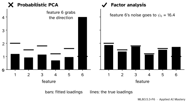
Last, factor analysis against probabilistic PCA, on six features driven by one hidden factor, where the sixth is measured with noise of standard deviation 4 instead of 0.5.
loadings = np.array([2.0, 1.5, 1.8, 1.2, 1.6, 1.0])rng = np.random.default_rng(7)z = rng.normal(size=300)Y = np.outer(z, loadings) + rng.normal(size=(300, 6)) * np.array([0.5, 0.5, 0.5, 0.5, 0.5, 4.0])w_pca = ppca(Y, 1)[1].ravel()fa = FactorAnalysis(n_components=1).fit(Y)w_fa = fa.components_[0] * np.sign(fa.components_[0][0])cos =lambda a, b: a @ b / np.linalg.norm(a) / np.linalg.norm(b)print("PPCA loadings:", w_pca.round(2), " match with the truth:", round(cos(w_pca, loadings), 2))print("FA loadings: ", w_fa.round(2), " match with the truth:", round(cos(w_fa, loadings), 2))print("FA noise variances:", fa.noise_variance_.round(2))print("held-out log-likelihood, PPCA and FA:",round(cross_val_score(PCA(1), Y, cv=5).mean(), 2), round(cross_val_score(FactorAnalysis(1), Y, cv=5).mean(), 2))
PPCA loadings: [1.17 0.9  1.12 0.68 0.93 3.98]   match with the truth: 0.69
FA loadings:   [1.85 1.35 1.74 1.12 1.49 1.7 ]   match with the truth: 0.98
FA noise variances: [ 0.22  0.23  0.21  0.27  0.23 16.44]
held-out log-likelihood, PPCA and FA: -11.78 -8.33
Probabilistic PCA puts its largest loading on the noisy sixth feature, because that feature has the largest variance and PPCA can only explain variance through \(\mat{W}\) or through one shared \(\sigma^2\). Factor analysis gives the sixth feature its own noise variance, about 16.4 against a true 16, and recovers loadings close to the truth.
Explore
The module’s interactive, variance and error, is in lesson ML03.5.1. Snap the line to the first direction: in the read-out, \(\lambda_2\) is the mean squared error left over. In this lesson’s language, for a two-feature cloud with \(q = 1\) that is exactly the fitted noise variance \(\sigma^2\), up to the factor \({(n - 1)/n}\).
Pitfalls
ML03.5.3-F6
Wrong beside right. One noisy feature drags probabilistic PCA’s direction towards itself; factor analysis absorbs the extra noise in that feature’s own variance.
“Probabilistic PCA and factor analysis are the same thing.”
They share the story but not the noise. PPCA assumes every feature is equally noisy, so a badly measured feature looks like signal and pulls \(\mat{W}\) towards itself. Factor analysis estimates one noise variance per feature. When features are on different scales or of different quality, factor analysis fits better; when the noise really is round, PPCA is simpler and has a closed form.
“The columns of \(\mat{W}\) are the principal directions.”
They point along them only for \({\mat{R} = \mat{I}}\), and even then they are scaled by \({\sqrt{\lambda_j - \sigma^2}}\), not of length 1. Any rotation \(\mat{R}\) fits equally well, so a fitted \(\mat{W}\) from an iterative method (EM, or factor analysis) can be any turned version. Compare subspaces, or the products \({\mat{W}\mat{W}\T}\), not raw columns.
“A higher training log-likelihood means a better \(q\).”
On the training data the likelihood can only rise as \(q\) grows, since a larger model contains the smaller one. Compare on held-out data, as cross_val_score with PCA.score does: there the 12-feature data peak at \({q = 3}\), the true number of factors.
Check yourself
Recall
1. What is the covariance of \(\vect{x}\) under probabilistic PCA?
Show answer
\({\mat{W}\mat{W}\T + \sigma^2\mat{I}}\).
2. In the maximum-likelihood fit, what is \(\sigma^2\)?
Show answer
The mean of the \({d - q}\) discarded eigenvalues of \(\mat{S}\): the average variance PCA throws away.
3. Why is \(\mat{W}\) only determined up to an orthogonal \(\mat{R}\)?
Show answer
Because \({\mat{W}\mat{R}(\mat{W}\mat{R})\T = \mat{W}\mat{W}\T}\), so the distribution of \(\vect{x}\) is unchanged; turning the hidden space cannot be seen in the data.
4. How does scikit-learn let you choose \(q\) with this model?
Show answer
PCA.score returns the average log-likelihood under the model; cross-validate it over \(q\) and keep the \(q\) with the best held-out score.
5. What does factor analysis change, and when does it help?
Show answer
The noise covariance becomes a diagonal \(\mat{\Psi}\), one variance per feature. It helps when features differ in how noisy they are.
Exercises
1.★ Data in \(\R^5\) have eigenvalues of \(\mat{S}\) equal to 10, 4, 0.5, 0.3 and 0.2. Fit probabilistic PCA with \({q = 2}\): give \(\sigma^2\) and the lengths of the two columns of \(\mat{W}\).
Show solution
\({\sigma^2 = (0.5 + 0.3 + 0.2)/3 = 1/3}\). The columns have lengths \({\sqrt{10 - 1/3} \approx 3.11}\) and \({\sqrt{4 - 1/3} \approx 1.91}\).
2.★★ Count the free parameters of probabilistic PCA with \(d = 64\) and \(q = 10\), and compare with a full Gaussian. Remember that \(\mat{R}\) removes some freedom from \(\mat{W}\).
Show solution
\(\vect{\mu}\) has 64, \(\sigma^2\) has 1, and \(\mat{W}\) has \({64 \times 10 = 640}\) entries, of which \({q(q - 1)/2 = 45}\) only choose the rotation \(\mat{R}\) and cannot be seen. That is \({64 + 640 - 45 + 1 = 660}\). A full Gaussian needs \({64 + 64 \times 65/2 = 2144}\). PPCA sits in between a round Gaussian (65) and a full one, which is why it can be fitted well from fewer examples.
3.★★★ Show that for \({q = d - 1}\) the fitted covariance equals \(\mat{S}\) exactly, and that \({\operatorname{tr}(\mat{\Sigma}^{-1}\mat{S}) = d}\) at the maximum for every \(q\).
Show solution
The fitted \(\mat{\Sigma}\) has eigenvectors \(\vect{u}_j\), with eigenvalue \(\lambda_j\) for \({j \le q}\) and \(\sigma^2\) for \({j > q}\). With \({q = d - 1}\) only \(\lambda_d\) is dropped, so \({\sigma^2 = \lambda_d}\) and every eigenvalue matches \(\mat{S}\)’s, with the same eigenvectors; hence \({\mat{\Sigma} = \mat{S}}\). For any \(q\), \(\mat{\Sigma}^{-1}\) and \(\mat{S}\) share eigenvectors, so \({\mat{\Sigma}^{-1}\mat{S}}\) has eigenvalues \({\lambda_j/\lambda_j = 1}\) for \({j \le q}\) and \({\lambda_j/\sigma^2}\) for \({j > q}\). Its trace is \({q + \sum_{j>q}\lambda_j/\sigma^2 = q + (d - q) = d}\), by the definition of \(\sigma^2\).
Summary card
PCA is the best fit of a story: a few Gaussian hidden numbers, a linear map, and round noise.
Factor analysis. Noise \({\mat{\Psi}}\) diagonal, one variance per feature.
Sources and next steps
Sources. Each was opened and checked against this lesson on 15 November 2026.
Michael E. Tipping and Christopher M. Bishop, Mixtures of probabilistic principal component analysers, Neural Computation 11 (1999), 443 to 482 (the authors’ copy). Section 2.2 is factor analysis with diagonal \(\mat{\Psi}\); Section 3 gives the model covariance \({\sigma^2\mat{I} + \mat{W}\mat{W}\T}\) (7), the log-likelihood (10) with \(\mat{S}\) dividing by \(N\) (11), the stationary points \({\mat{U}_q(\mat{\Lambda}_q - \sigma^2\mat{I})^{1/2}\mat{R}}\) (14) with the global maximum at the principal eigenvectors, \({\sigma^2_{\text{ML}}}\) as the mean of the discarded eigenvalues (15), and the posterior mean \({\mat{M}^{-1}\mat{W}\T(\vect{t} - \vect{\mu})}\) in Section 3.3. The paper writes \(\vect{t}\) for the data and \(\vect{x}\) for the latent variable.
Christopher M. Bishop, Pattern Recognition and Machine Learning, Section 12.2.1 (equations 12.44 to 12.46, and the reading of \(\lambda_i - \sigma^2\) as the variance carried by the latent space) and Section 12.2.4 on factor analysis.
scikit-learn 1.9, sklearn.decomposition.PCA: noise_variance_ follows Tipping and Bishop and equals the average of the smallest eigenvalues of the covariance; score returns the average log-likelihood. FactorAnalysis and the User Guide, Section 2.5.5: a diagonal noise covariance gives factor analysis, an isotropic one gives probabilistic PCA.
Next.ML03.5.4 Kernel PCA stays with eigenvectors but bends the space first, so that PCA can follow curved structure.