Single linkage is a minimum spanning tree in disguise. Prove that Kruskal’s algorithm adds edges in the order single linkage merges, see why that makes single linkage fast and fragile, and meet bisecting k-means and connectivity constraints for larger data.
ML03.2.4L2 Intermediate30 minIn review (what this means)
The maths and code on this page are checked by automated tests on every change, but an independent reader has not signed it off yet. Spot a mistake or a confusing step? Tell us.
Prove that Kruskal’s algorithm adds the edges of a minimum spanning tree in the order and at the heights at which single linkage merges.
Get single linkage’s K clusters by removing the K − 1 longest edges of the minimum spanning tree, from scratch and with scipy.sparse.csgraph.
Explain why single linkage is fast and fragile, using a bridge point, and how HDBSCAN’s mutual reachability distance repairs it.
Cluster larger data top-down with BisectingKMeans, and with connectivity constraints in AgglomerativeClustering.
Name where hierarchies are used in practice: taxonomies and clustered heatmaps of gene expression.
The question
The direct method of ML03.2.1 takes about \({n^3/6}\) steps, which rules out a million points. Yet single linkage, the most fragile of the linkages, is the one that libraries can run fastest. Why is single linkage special, and what can be done with the others when the data are large?
From the last lesson
1. What is the cophenetic distance between two points?
Show answer
The height of the merge at which the two points first share a cluster.
2. What does t mean in fcluster(Z, t, criterion="maxclust")?
Show answer
The largest number of clusters wanted: SciPy finds the lowest cut with at most t clusters.
Intuition
Think of the points as towns and the distances as the lengths of possible roads. Build the cheapest road network that connects every town: a minimum spanning tree. Its roads are the single-linkage merges, length for length.
ML03.2.4-F1
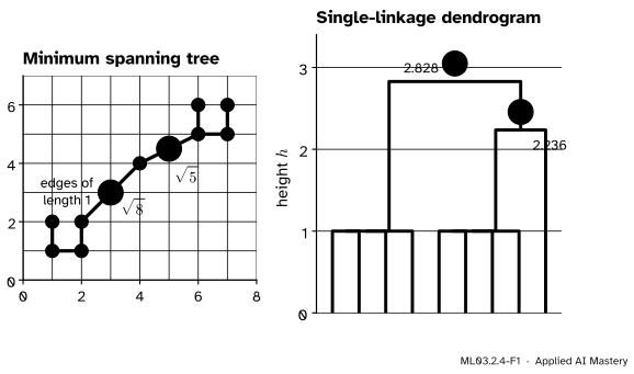
The minimum spanning tree of the nine points (left) and their single-linkage dendrogram (right). The tree’s edges, sorted, are the merge heights: six of length 1, then \({\sqrt{5} \approx 2.236}\) and \({\sqrt{8} \approx 2.828}\).
A single-linkage merge joins two clusters through their closest pair of points. Keep that pair as an edge. After \({n - 1}\) merges the edges join every point, never close a loop, and each was the shortest available: a minimum spanning tree.
Build it up
Step 1. A graph. Make each point a node and join every pair by an edge whose weight is their distance \(d_{ij}\). This complete graph has \({n(n - 1)/2}\) edges.
Step 2. A spanning tree. A spanning tree is a set of edges that connects all \(n\) nodes and contains no cycle. Every spanning tree has exactly \({n - 1}\) edges. A minimum spanning tree (MST) is one with the smallest total weight.
Step 3. Kruskal’s algorithm. Go through the edges from shortest to longest. Add an edge if its two ends are in different pieces of the forest built so far; skip it if they are already connected, since it would close a cycle. Stop at \({n - 1}\) edges. Kruskal’s algorithm returns a minimum spanning tree.
ML03.2.4-F2
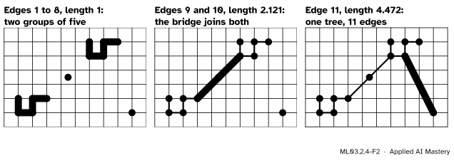
Kruskal’s algorithm on the twelve points. The pieces of the growing forest are the clusters of single linkage at the same stage.
Step 4. Cutting the tree. Remove the longest edge of the MST and it falls into two pieces: the last single-linkage merge, undone. Remove the \({K - 1}\) longest edges and you have \(K\) pieces, the single-linkage clusters for \(K\).
The formal statement
NoteTheorem: single linkage is Kruskal’s algorithm
Let Kruskal’s algorithm, run on the complete graph of the points with weights \(d_{ij}\), add the edges \({e_1, \dots, e_{n-1}}\) with weights \({w_1 \le \dots \le w_{n-1}}\). If at every step the shortest available edge is unique, then for every \(t\):
the pieces of the forest \({\{e_1, \dots, e_t\}}\) are the clusters of single linkage after \(t\) merges, and
the \(t\)-th single-linkage merge height is \({h_t = w_t}\).
Corollary. Removing the \({K - 1}\) longest edges of the MST leaves \(K\) pieces, and they are the single-linkage clusters for \(K\).
Proof, by induction on \(t\). For \({t = 0}\) both sides are the \(n\) single points.
Suppose both statements hold after \(t\) steps, so Kruskal’s pieces are the current clusters \({C_1, \dots, C_{n-t}}\). Kruskal looks at edges in increasing order and skips an edge only if its ends are already in one piece. Every edge examined so far has both ends in one piece now: it was either added, or skipped because its ends were already connected. So the next edge Kruskal adds is the shortest edge whose two ends lie in different pieces. Its weight is
where the first minimum runs over pairs of different pieces. The inner minimum is the single-linkage distance between \(C_a\) and \(C_b\), so the right-hand side is the smallest single-linkage distance between two current clusters. That is precisely the pair single linkage merges next, at height \({h_{t+1} = w_{t+1}}\). Kruskal’s new edge joins exactly those two clusters, so after step \({t + 1}\) the pieces are again the clusters. \(\square\)
The corollary follows. Keeping the \({n - K}\) shortest MST edges is stopping Kruskal after \({n - K}\) steps, which by the theorem gives the clusters after \({n - K}\) merges, that is, \(K\) clusters. (With ties, both methods may break them differently. The heights still agree, but at a tied height the clusters for one \(K\) can differ, as the twelve points will show.)
Why this makes single linkage fast. The MST can be found without the \({n^3/6}\) scans of the direct method. Jarník’s (or Prim’s) algorithm grows one tree from a start point; with a suitable priority queue it runs in time of order \({E + V \log V}\) for \(V\) nodes and \(E\) edges, which on the complete graph of \(n\) points is of order \(n^2\). SciPy’s linkage documents an MST-based algorithm of order \(n^2\) for single linkage (and a “nearest-neighbours chain” algorithm, also \(n^2\), for complete, average and Ward). All of them still need memory of order \(n^2\) for the distances.
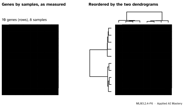
Where hierarchies are used. Taxonomies (species within genera within families) are hierarchies, and clustering genes is a standard first look at expression data. A clustered heatmap orders the rows and columns of a data matrix by the leaf orders of their own dendrograms, so similar genes and samples sit side by side, as in ESL’s Figure 14.14.
ML03.2.4-F6
A clustered heatmap of invented expression values. The two dendrograms only reorder the rows and the columns, yet the block structure that was hidden by the measured order appears.
Worked example
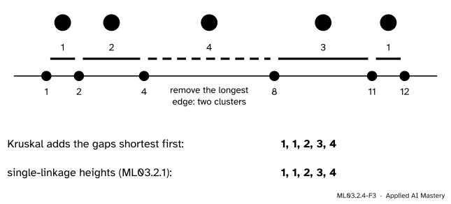
On a line, the MST is the gaps. For the six values 1, 2, 4, 8, 11, 12, an edge between two values that are not neighbours is longer than each gap it spans, and the five gaps between neighbours already connect everything. So the MST is the five gaps, 1, 2, 4, 3, 1, and Kruskal adds them in the order 1, 1, 2, 3, 4: exactly the single-linkage heights of ML03.2.1.
ML03.2.4-F3
On a line the minimum spanning tree is the chain of gaps between neighbours. Removing the longest gap, 4, splits the values into \({\{1, 2, 4\}}\) and \({\{8, 11, 12\}}\).
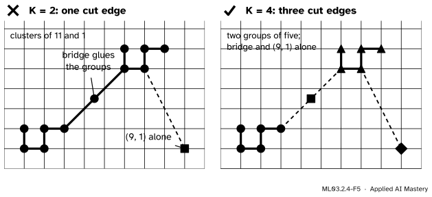
The twelve points. The MST has eleven edges: eight of length 1 inside the two groups of five, two of length \({\sqrt{4.5} \approx 2.121}\) from the bridge \({(4.5, 3.5)}\) to \({(3, 2)}\) and to \({(6, 5)}\), and one of length \({\sqrt{20} \approx 4.472}\) from \({(9, 1)}\) to \({(7, 5)}\).
\({K = 2}\): remove the longest edge. The pieces are \({\{(9, 1)\}}\) and the other eleven points.
\({K = 3}\): the next longest edges tie at 2.121, so there is no single answer: the bridge stays with one group or the other, depending on which tied edge is removed.
\({K = 4}\): remove all three long edges. The pieces are the two groups of five, the bridge alone and \({(9, 1)}\) alone.
With \({K = 4}\), single linkage matches DBSCAN on these points (ML03.3.1): two clusters of five and two points that belong to neither.
Code
Kruskal’s algorithm from scratch, with a small union-find structure that remembers which piece each point is in.
import numpy as npfrom scipy.cluster.hierarchy import fcluster, linkagefrom scipy.spatial.distance import pdist, squareformtwelve = np.array([(1, 1), (2, 1), (1, 2), (2, 2), (3, 2), (6, 5), (7, 5), (6, 6), (7, 6), (8, 6), (4.5, 3.5), (9, 1)])def kruskal(X): D = squareform(pdist(X)) n =len(X) edges =sorted((D[i, j], i, j) for i inrange(n) for j inrange(i +1, n)) parent =list(range(n))def find(a):while parent[a] != a: a = parent[a]return a tree = []for w, i, j in edges: ri, rj = find(i), find(j)if ri != rj: # different pieces: the edge is safe parent[ri] = rj tree.append((float(w), i, j))iflen(tree) == n -1:breakreturn treemst = kruskal(twelve)weights = [w for w, _, _ in mst]print("MST edge lengths:", np.round(weights, 3))print("single linkage: ", np.round(linkage(twelve, "single")[:, 2], 3))
SciPy has the MST built in. Cutting its \({K - 1}\) longest edges and asking for the connected pieces gives the clusters, which match fcluster:
from scipy.sparse.csgraph import connected_components, minimum_spanning_treeT = minimum_spanning_tree(squareform(pdist(twelve))).toarray()print("SciPy's MST, total length:", round(T.sum(), 3))def mst_clusters(T, K): W = T.copy()for _ inrange(K -1): # remove the K - 1 longest edges W[np.unravel_index(np.argmax(W), W.shape)] =0return connected_components(W, directed=False)[1]Z = linkage(twelve, "single")for K in (2, 4): ours = mst_clusters(T, K)print(f"K = {K}: sizes {sorted(np.bincount(ours).tolist())},","same as fcluster:", len(set(zip(ours, fcluster(Z, K, criterion="maxclust")))) == K)
SciPy's MST, total length: 16.715
K = 2: sizes [1, 11], same as fcluster: True
K = 4: sizes [1, 1, 5, 5], same as fcluster: True
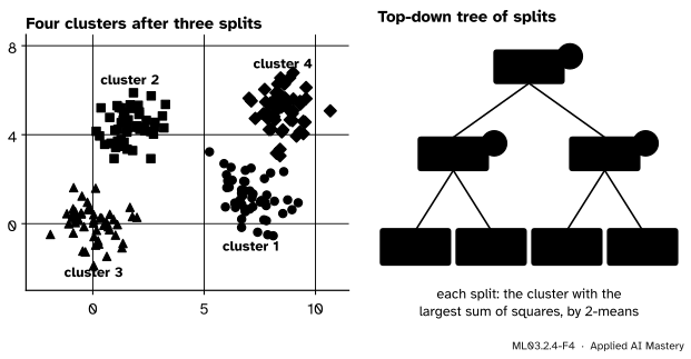
For larger data, two tools from scikit-learn. Bisecting k-means works top-down: start with one cluster and repeatedly split one cluster in two with 2-means. By default it splits the cluster with the largest sum of squares (bisecting_strategy="biggest_inertia"), and each split only touches the points of one cluster. Here it is from scratch beside BisectingKMeans, on four seeded blobs:
cluster sizes: [50, 50, 50, 50] same partition: True
ML03.2.4-F4
Bisecting k-means on four blobs. The first split separates left from right; each later split cuts the cluster with the largest sum of squares. The splits form a top-down tree.
Connectivity constraints let agglomerative clustering merge only clusters that are neighbours in a given graph, such as the 10-nearest-neighbour graph. scikit-learn’s guide notes that this imposes local structure and makes the algorithm faster for large \(n\). On two seeded half-moons:
from sklearn.cluster import AgglomerativeClusteringfrom sklearn.datasets import make_moonsfrom sklearn.neighbors import kneighbors_graphXm, moon = make_moons(n_samples=300, noise=0.06, random_state=0)graph = kneighbors_graph(Xm, n_neighbors=10, include_self=False)agree = {}for method in ["average", "ward"]:for name, conn in [("free", None), ("10-NN graph", graph)]: labels = AgglomerativeClustering(n_clusters=2, linkage=method, connectivity=conn).fit(Xm).labels_ same =max(np.sum(labels == moon), np.sum(labels != moon)) agree[method, name] =int(same)print(f"{method:8s}{name:12s}: {same} of 300 points on their own moon's side")
average  free        : 248 of 300 points on their own moon's side
average  10-NN graph : 298 of 300 points on their own moon's side
ward     free        : 232 of 300 points on their own moon's side
ward     10-NN graph : 232 of 300 points on their own moon's side
With the graph, average linkage follows the moons (298 of 300); without it, it cuts across them (248). Ward’s rule still prefers round clusters either way (232). Single linkage, run on its own, separates the two moons perfectly here: on thin, well-separated shapes its chaining is a strength.
Explore
Load the twelve points in the dendrogram cutter of lesson ML03.2.3 with single linkage. Cut into two clusters and see \({(9, 1)}\) split off alone; then switch to average or Ward linkage and watch the two groups separate instead. Drag the bridge point away and the single-linkage tree changes at once.
Pitfalls
ML03.2.4-F5
Wrong beside right. Cut into two, single linkage splits off one outlying point and glues both groups together through the bridge. Cut the three longest edges and the two groups appear, with the bridge and the outlier on their own.
“Single linkage with K = 2 finds the two groups.”
One bridge point joins two groups at the height of its two short edges, 2.121 here, so the longest MST edges are the ones to outliers. Look at all the long edges, as \({K = 4}\) does, or use a method built for this. HDBSCAN (ML03.3.4) replaces \(d_{ij}\) by the mutual reachability distance, the largest of \(\text{core}_k(i)\), \(\text{core}_k(j)\) and \(d_{ij}\), where \({\text{core}_k(i)}\) is the distance from \(i\) to its \(k\)-th nearest neighbour. A point in a sparse place, like the bridge, has a large core distance, so all its edges are stretched and single linkage no longer chains through it. scikit-learn’s guide describes HDBSCAN as a minimum spanning tree of the mutual reachability graph, cut at its longest edges.
“A fast algorithm for single linkage means hierarchical clustering scales.”
The \(n^2\) algorithms remove the \(n^3\) time, not the \(n^2\) memory: SciPy states that all its linkage algorithms use memory of order \(n^2\), and the distances of a million points would not fit. For large data, cluster a sample, restrict merges to a sparse neighbour graph, or go top-down with bisecting k-means, which never forms all the distances.
“Bisecting k-means gives the same tree as agglomerative clustering, just upside down.”
Each split is a greedy 2-means run that can depend on its start, and an early split is never revisited. ESL notes that recursive 2-means splitting need not even give the monotone heights a dendrogram requires. It is a fast route to a few clusters, not the full bottom-up tree.
Check yourself
Recall
1. What is a minimum spanning tree?
Show answer
A set of \({n - 1}\) edges that connects all the points without a cycle and has the smallest total length among all such sets.
2. How does Kruskal’s algorithm build it?
Show answer
It goes through the edges from shortest to longest and adds an edge whenever its two ends are in different pieces of the forest built so far, until \({n - 1}\) edges are chosen.
3. How do you get the single-linkage clusters for \(K\) from the MST?
Show answer
Remove the \({K - 1}\) longest edges; the \(K\) connected pieces that remain are the clusters.
4. On the twelve points, what does single linkage give for \({K = 2}\), and why?
Show answer
\({(9, 1)}\) alone and the other eleven together, because the bridge \({(4.5, 3.5)}\) joins the two groups at 2.121, while \({(9, 1)}\) is 4.472 from its nearest neighbour.
5. What is the mutual reachability distance used by HDBSCAN?
Show answer
The largest of \(\text{core}_k(i)\), \(\text{core}_k(j)\) and \(d_{ij}\): the distance, raised to at least the core distance of each point, so that points in sparse places are pushed away from everyone.
Exercises
1.★ Find the MST of the values 0, 3, 4, 9, 10 and use it to give the single-linkage heights and the clusters for \({K = 2}\) and \({K = 3}\).
Show solution
On a line the MST is the chain of gaps between neighbours: 3, 1, 5, 1. Sorted, the single-linkage heights are 1, 1, 3, 5. For \({K = 2}\) remove the longest gap, 5, between 4 and 9: \({\{0, 3, 4\}}\) and \({\{9, 10\}}\). For \({K = 3}\) remove 5 and 3: \(\{0\}\), \({\{3, 4\}}\), \({\{9, 10\}}\).
2.★★ Without the uniqueness assumption the theorem’s first statement can fail for one \(K\). Explain what happens on the twelve points for \({K = 3}\), and why the merge heights still agree.
Show solution
The two edges from the bridge, to \({(3, 2)}\) and to \({(6, 5)}\), both have length \(\sqrt{4.5}\). Kruskal may add either first, and single linkage may merge the bridge with either group first. After nine merges the clusters are the bridge with one group of five, the other group, and \({(9, 1)}\), and which group the bridge has joined depends on how the tie was broken. The heights cannot differ: each method takes the smallest available distance at each step, and both available distances here are \(\sqrt{4.5}\), so the sorted heights are the same whichever is taken first.
3.★★★ Prove that every spanning tree of \(n\) points has exactly \({n - 1}\) edges. Then use it to explain why, after \(t\) steps of Kruskal’s algorithm, there are exactly \({n - t}\) pieces.
Show solution
Start with the \(n\) points and no edges: \(n\) pieces. Adding an edge between two different pieces joins them, so the number of pieces falls by exactly one; adding an edge inside one piece would close a cycle. A spanning tree has no cycle, so each of its edges, added one at a time in any order, joins two different pieces. It ends with one piece (it connects everything), so it took \({n - 1}\) edges to go from \(n\) pieces to 1. Kruskal only ever adds edges between different pieces, so after \(t\) additions the count has fallen from \(n\) to \({n - t}\), matching the \({n - t}\) clusters of single linkage after \(t\) merges.
Summary card
Single linkage is the minimum spanning tree: sort its edges for the heights, cut the longest for the clusters.
\(K\) clusters: remove the \({K - 1}\) longest MST edges.
Fast but fragile: about \(n^2\) time, \(n^2\) memory; one bridge point chains two groups.
Repairs and scale: HDBSCAN’s mutual reachability; BisectingKMeans; connectivity= graphs.
Sources and next steps
Sources. Each was opened and checked against this lesson on 15 November 2026.
J. Erickson, Algorithms, 2019, Chapter 7, Minimum spanning trees, section on Kruskal’s algorithm: scan all edges by increasing weight and add an edge if it is safe, which, in that order, means its endpoints lie in different components of the forest; sorting the edges dominates the running time. The same chapter gives Jarník’s (“Prim’s”) algorithm a running time of \({O(E + V \log V)}\) with a Fibonacci heap.
SciPy developers, scipy.cluster.hierarchy.linkage: an algorithm based on the minimum spanning tree for single linkage and the nearest-neighbours chain for complete, average, weighted and Ward, both of order \(n^2\) in time, and memory of order \(n^2\) for all algorithms. And scipy.sparse.csgraph.minimum_spanning_tree: it returns the tree as an \({N \times N}\) sparse matrix, and a zero entry of a dense input means no edge.
scikit-learn developers, User Guide, Section 2.3: Clustering (version 1.9). Section 2.3.6: connectivity constraints from kneighbors_graph, which impose local structure and make the algorithm faster; single linkage as efficient but not robust to noise, and good on non-globular data. Section 2.3.6.5: bisecting k-means and its two bisecting strategies. Section 2.3.8: HDBSCAN’s core distance, mutual reachability distance and minimum spanning tree of the mutual reachability graph.
T. Hastie, R. Tibshirani and J. Friedman, The Elements of Statistical Learning, 2nd edition, 12th printing. Section 14.3.12: divisive clustering by recursive 2-means and its lack of the monotonicity a dendrogram needs; Figure 14.14, rows and columns of a microarray ordered by average-linkage clustering.
Next. The next module of the course, ML03.3 Density-based clustering, finds clusters as dense regions with DBSCAN, OPTICS and HDBSCAN, the single-linkage tree done right. Module ML03.10 asks how to judge any of these clusterings.