\( \newcommand{\vect}[1]{\boldsymbol{\mathbf{#1}}} \newcommand{\mat}[1]{\boldsymbol{\mathbf{#1}}} \newcommand{\R}{\mathbb{R}} \newcommand{\E}{\mathbb{E}} \newcommand{\Prob}{\mathbb{P}} \newcommand{\T}{^{\top}} \newcommand{\norm}[1]{\lVert #1 \rVert} \newcommand{\abs}[1]{\lvert #1 \rvert} \newcommand{\ihat}{\mkern1mu\hat{\boldsymbol{\imath}}\mkern2mu} \newcommand{\jhat}{\mkern1mu\hat{\boldsymbol{\jmath}}\mkern2mu} \newcommand{\pd}[2]{\frac{\partial #1}{\partial #2}} \newcommand{\argmax}{\operatorname*{arg\,max}} \newcommand{\argmin}{\operatorname*{arg\,min}} \newcommand{\cdata}[1]{\class{c-data}{#1}} \newcommand{\cmodel}[1]{\class{c-model}{#1}} \newcommand{\ctruth}[1]{\class{c-truth}{#1}} \newcommand{\cgrad}[1]{\class{c-grad}{#1}} \newcommand{\closs}[1]{\class{c-loss}{#1}} \newcommand{\cparam}[1]{\class{c-param}{#1}} \newcommand{\csecond}[1]{\class{c-second}{#1}} \renewcommand{\,}{\mkern3mu} \)

Forward or reverse: cost and memory

Forward mode builds a Jacobian a column per sweep and reverse mode a row per sweep: the two orders of multiplying a chain of Jacobians. Count the work on a chain of three Jacobians, see why a gradient costs a few runs of the model, what reverse mode pays in memory, and how Hessian-vector products combine the two modes.

M05.8.4L2 Intermediate25 min

In review

The maths and code on this page are checked by automated tests on every change, but an independent reader has not signed it off yet. Spot a mistake or a confusing step? Tell us.

Before this lesson: M05.8.3 Reverse mode: adjoints and the tape

What you will be able to do

Explain forward and reverse mode as the two orders of multiplying a chain of Jacobians, right to left and left to right.
Count the multiplications of both orders for a chain of Jacobians and choose the cheaper mode from the numbers of inputs and outputs.
Explain why reverse mode gives a gradient for a small constant times the cost of one run, and why it must store the forward trace.
Sketch how a Hessian-vector product is computed by forward mode over the reverse-mode gradient.

The question

Forward mode and reverse mode compute exactly the same derivatives. Forward mode is simpler and needs no tape; reverse mode must remember everything. So why does every deep-learning library use reverse mode for training, and are there jobs where forward mode is the better choice?

From the last lesson

1. What is the adjoint \(\delta_v\) of a variable, and where does the backward sweep start?

Show answer

\({\delta_v = \partial y/\partial v}\), the derivative of the output with respect to \(v\). The sweep starts with \({\delta_y = 1}\) at the output.

2. Why must adjoints be added when a value is used twice?

Show answer

The chain rule on a graph sums over all paths to the output, and a value used twice starts paths along each of its uses; one contribution comes back along each.

Intuition

A program that runs in stages is a composition, and the Jacobian of a composition is the product of the stages’ Jacobians (M05.4.3): for three stages, \({\mat{J}_f = \mat{A}\mat{B}\mat{C}}\), with \(\mat{C}\) the Jacobian of the first stage and \(\mat{A}\) of the last. Matrix multiplication is associative, so \({(\mat{A}\mat{B})\mat{C}}\) and \({\mat{A}(\mat{B}\mat{C})}\) are the same matrix. They are not the same amount of work.

M05.8.4-F1

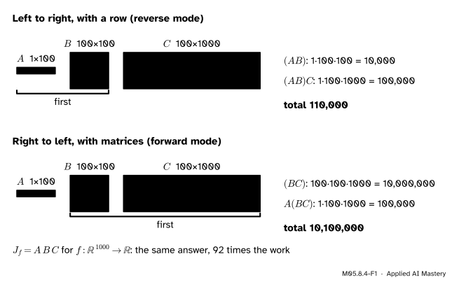
The Jacobian of a function with 1000 inputs and one output, as a chain of three stages. Multiplied from the left, every intermediate result is a single row; multiplied from the right, the first product is a 100 by 1000 matrix.

Reverse mode multiplies from the left, starting at the output. With one output, the leftmost factor is a row, so every partial product stays a row and every step is cheap. Forward mode multiplies from the right, starting at the inputs, where the “vector” is really \(n\) seed vectors, one per input. With 1000 inputs that is 1000 columns to push through.

Build it up

Step 1. The cost of one product. Multiplying an \({m \times q}\) matrix by a \({q \times p}\) matrix takes \(mp\) dot products of length \(q\): \({m\,q\,p}\) multiplications.

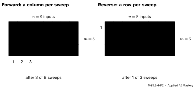
Step 2. Forward mode is right to left, a column at a time. The seed \(\vect{e}_j\) asks for \({\mat{J}_f\vect{e}_j = \mat{A}(\mat{B}(\mat{C}\vect{e}_j))}\): each stage applies its Jacobian to the tangent vector it receives. One sweep gives column \(j\); the whole Jacobian takes \(n\) sweeps. Done for all \(j\) at once, this is the product \({\mat{A}(\mat{B}\mat{C})}\).

Step 3. Reverse mode is left to right, a row at a time. Seeding the output adjoints with \(\vect{u}\) asks for \({\vect{u}\T\mat{J}_f = ((\vect{u}\T\mat{A})\mat{B})\mat{C}}\): each stage multiplies the row of adjoints by its Jacobian (M05.8.3, exercise 3). One sweep gives one row; the whole Jacobian takes \(m\) sweeps.

M05.8.4-F2

The same Jacobian, filled in two ways. Forward mode needs as many sweeps as there are inputs, reverse mode as many as there are outputs.

Step 4. Reverse mode must look ahead. To start from the left, it needs \(\mat{A}\), the Jacobian of the last stage. But \(\mat{A}\) depends on the values that reach the last stage, and those exist only after the first two stages have run. So reverse mode runs the whole program forward first and stores every value that a local derivative will need: the tape of M05.8.3. Forward mode travels in the same direction as the program, and can throw each value away once the next stage has used it.

The formal statement

Cost of the two modes

Let \({f : \R^n \to \R^m}\) be a program that costs \({\text{ops}(f)}\) elementary operations, and let \(c\) be the small constant factor by which a sweep with derivatives is dearer than a plain run.

A forward sweep gives one column \({\mat{J}_f\vect{r}}\); the full Jacobian costs about \({n \cdot c \cdot \text{ops}(f)}\).
A reverse sweep gives one row \({\vect{u}\T\mat{J}_f}\); the full Jacobian costs about \({m \cdot c \cdot \text{ops}(f)}\), and its memory grows, in the worst case, with \({\text{ops}(f)}\), because the trace is stored.

For a loss, \({m = 1}\), and reverse mode gives the whole gradient for about \({c \cdot \text{ops}(f)}\), whatever \(n\) is.

Baydin et al. state the constant as \({c < 6}\), and typically 2 to 3, following Griewank and Walther’s book on the subject. Where it comes from: each elementary step does its own work once in the forward pass, and in the backward pass does one multiply-add per input edge, with local derivatives that cost about as much as the step itself. A dense layer is the clearest case: its forward pass is one matrix product, its backward pass two of the same size (M05.9.4).

Which to use. Count inputs and outputs. Training a model has millions of inputs (the weights) and one output (the loss): reverse mode, by a factor of about \(n\). A function with few inputs and many outputs, such as a curve \({f : \R \to \R^{1000}}\) or the sensitivity of a whole simulation to one parameter, wants forward mode. When \({n = m}\), neither has the advantage of scale, and forward mode is often preferred because it needs no tape. Bright, Edelman and Johnson note that in practice forward mode can win even for many inputs and one output until \(n\) is fairly large, perhaps over 100, because the bookkeeping of reverse mode has its own cost.

Memory and its remedy. The tape holds every intermediate value of the forward pass. For a deep network, that means every activation of every layer for the whole batch, and memory, not arithmetic, is often what limits the batch size. Checkpointing keeps only some of the values and recomputes the rest during the backward pass, trading time for memory (M05.9.4).

Second derivatives: Hessian-vector products. Newton-type methods and the study of curvature need \({\mat{H}\vect{v}}\), the Hessian times a vector. Since the Hessian is the Jacobian of the gradient, and a Jacobian-vector product is one forward sweep,

\[ \mat{H}_f(\vect{x})\,\vect{v} = \frac{d}{d\alpha}\, \nabla f(\vect{x} + \alpha\vect{v}) \Big|_{\alpha = 0} . \]

So: write the reverse-mode gradient as a program, and run that program on dual numbers \({x_j + v_j\,\varepsilon}\). The values give \(\nabla f\), the \(\varepsilon\) parts give \({\mat{H}\vect{v}}\). This is forward over reverse. It costs a constant times one gradient, and never forms the \({n \times n}\) Hessian. (Baydin et al. describe the mirror image, reverse mode applied to a forward-mode directional derivative; both give \({\mat{H}\vect{v}}\).)

Worked example

Three stages: 1000 inputs, 100, 100, one output. The Jacobians are \({\mat{C}\ (100 \times 1000)}\), \({\mat{B}\ (100 \times 100)}\) and \({\mat{A}\ (1 \times 100)}\), so \({\mat{J}_f = \mat{A}\mat{B}\mat{C}}\) is \({1 \times 1000}\): the gradient, written as a row.

Left to right (reverse mode). First \({\mat{A}\mat{B}}\): \({1 \cdot 100 \cdot 100 = 10{,}000}\) multiplications, giving a \({1 \times 100}\) row. Then that row times \(\mat{C}\): \({1 \cdot 100 \cdot 1000 = 100{,}000}\). Total 110,000.

Right to left (forward mode). First \({\mat{B}\mat{C}}\): \({100 \cdot 100 \cdot 1000 = 10{,}000{,}000}\), giving a \({100 \times 1000}\) matrix. Then \(\mat{A}\) times it: \({1 \cdot 100 \cdot 1000 = 100{,}000}\). Total 10,100,000, about 92 times as much. Read as sweeps, these are 1000 forward sweeps, one per input, each pushing a column of \(\mat{C}\) through \(\mat{B}\) (10,000) and then \(\mat{A}\) (100).

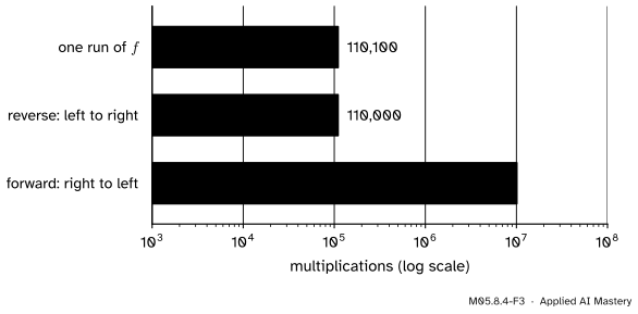
One run of \(f\) itself, with matrix-vector products: \({\mat{C}\vect{x}}\) costs 100,000, then \(\mat{B}\) 10,000 and \(\mat{A}\) 100, so 110,100. The reverse-mode gradient costs about the same again: the whole gradient for the price of about two runs.

M05.8.4-F3

The worked counts. The gradient by reverse mode costs about as much as one run of \(f\); by forward mode, about 92 runs.

The other shape. Turn the function round: one input and 1000 outputs, with Jacobians \({1000 \times 100}\), \({100 \times 100}\) and \({100 \times 1}\). Right to left, the first product costs \({100 \cdot 100 \cdot 1}\) and the second \({1000 \cdot 100 \cdot 1}\); left to right, the first costs \({1000 \cdot 100 \cdot 100}\) and the second \({1000 \cdot 100 \cdot 1}\):

\[ \begin{aligned} \text{right to left: } & 10{,}000 + 100{,}000 \\ &= 110{,}000, \\ \text{left to right: } & 10{,}000{,}000 + 100{,}000 \\ &= 10{,}100{,}000 . \end{aligned} \]

Forward mode wins by the same factor. The rule is the shape, not the mode.

Code

First the matrix-chain counts, then the two automatic-differentiation classes of the last two lessons, with a counter added to every operation. The classes are collapsed below; they are the same code as before, cut down to the operations needed here.

def cost(p, q):
    """Multiplications to multiply a matrix of shape p by a matrix of shape q."""
    assert p[1] == q[0], "shapes do not match"
    return p[0] * p[1] * q[1]

A, B, C = (1, 100), (100, 100), (100, 1000)
left_to_right = cost(A, B) + cost((A[0], B[1]), C)
right_to_left = cost(B, C) + cost(A, (B[0], C[1]))
one_run = C[0] * C[1] + B[0] * B[1] + A[0] * A[1]
print(f"left to right {left_to_right:,}, right to left {right_to_left:,}, one run {one_run:,}")
print(f"ratio {right_to_left / left_to_right:.1f}")

left to right 110,000, right to left 10,100,000, one run 110,100
ratio 91.8

The Dual and Var classes, with an operation counter

import math

COUNT = {"ops": 0}

class Dual:
    def __init__(self, value, tangent=0.0):
        self.value, self.tangent = value, tangent
    @staticmethod
    def lift(x):
        return x if isinstance(x, Dual) else Dual(x)
    def __add__(self, other):
        COUNT["ops"] += 1
        o = Dual.lift(other)
        return Dual(self.value + o.value, self.tangent + o.tangent)
    __radd__ = __add__
    def __neg__(self):
        return Dual(-self.value, -self.tangent)
    def __sub__(self, other):
        return self + (-Dual.lift(other))
    def __mul__(self, other):
        COUNT["ops"] += 1
        o = Dual.lift(other)
        return Dual(self.value * o.value, self.tangent * o.value + self.value * o.tangent)
    __rmul__ = __mul__
    def __truediv__(self, other):
        o = Dual.lift(other)
        return Dual(self.value / o.value, (self.tangent * o.value - self.value * o.tangent) / o.value ** 2)
    def __rtruediv__(self, other):
        return Dual.lift(other) / self

class Var:
    def __init__(self, value, parents=()):
        self.value, self.parents, self.adjoint = value, parents, 0.0
    @staticmethod
    def lift(x):
        return x if isinstance(x, Var) else Var(x)
    def __add__(self, other):
        COUNT["ops"] += 1
        o = Var.lift(other)
        return Var(self.value + o.value, ((self, 1.0), (o, 1.0)))
    __radd__ = __add__
    def __mul__(self, other):
        COUNT["ops"] += 1
        o = Var.lift(other)
        return Var(self.value * o.value, ((self, o.value), (o, self.value)))
    __rmul__ = __mul__
    def backward(self):
        order, seen, stack = [], set(), [(self, False)]
        while stack:
            v, finished = stack.pop()
            if finished:
                order.append(v)
            elif id(v) not in seen:
                seen.add(id(v))
                stack.append((v, True))
                stack += [(p, False) for p, _ in v.parents if id(p) not in seen]
        self.adjoint = 1.0
        for v in reversed(order):
            for parent, local in v.parents:
                COUNT["ops"] += 1                     # one multiply-add per edge
                parent.adjoint += v.adjoint * local

def sin(x):
    COUNT["ops"] += 1
    if isinstance(x, Dual):
        return Dual(math.sin(x.value), math.cos(x.value) * x.tangent)
    if isinstance(x, Var):
        return Var(math.sin(x.value), ((x, math.cos(x.value)),))
    return math.sin(x)

def cos(x):
    if isinstance(x, Dual):
        return Dual(math.cos(x.value), -math.sin(x.value) * x.tangent)
    return math.cos(x)

def ln(x):
    if isinstance(x, Dual):
        return Dual(math.log(x.value), x.tangent / x.value)
    return math.log(x)

A test function with \(n\) inputs, \({f(\vect{x}) = \sum_i \sin(x_i)\,x_{i-1}}\) (indices wrap round), costs three operations per input: a sine, a product and an addition. The full gradient by \(n\) forward sweeps, then by one reverse sweep:

import time
import numpy as np

def f(x):
    return sum(sin(x[i]) * x[i - 1] for i in range(len(x)))

rng = np.random.default_rng(0)
rows = []
for n in (1, 10, 100, 1000):
    x = rng.uniform(-1, 1, size=n)
    COUNT["ops"] = 0
    f([Dual(v) for v in x])                             # every tangent 0: the operations of a plain run
    run = COUNT["ops"]

    COUNT["ops"] = 0
    start = time.perf_counter()
    forward = [f([Dual(v, 1.0 if i == j else 0.0) for i, v in enumerate(x)]).tangent for j in range(n)]
    forward_time, forward_ops = time.perf_counter() - start, COUNT["ops"]

    COUNT["ops"] = 0
    start = time.perf_counter()
    xs = [Var(v) for v in x]
    f(xs).backward()
    reverse = [v.adjoint for v in xs]
    reverse_time, reverse_ops = time.perf_counter() - start, COUNT["ops"]

    rows.append((n, run, forward_ops, reverse_ops, np.max(np.abs(np.subtract(forward, reverse)))))
    print(f"n = {n:4d}: run {run:5d} ops | forward {forward_ops:9,d} ops, {forward_time:7.4f} s"
          f" | reverse {reverse_ops:6,d} ops, {reverse_time:7.4f} s")

n =    1: run     3 ops | forward         3 ops,  0.0000 s | reverse      8 ops,  0.0000 s
n =   10: run    30 ops | forward       300 ops,  0.0001 s | reverse     80 ops,  0.0000 s
n =  100: run   300 ops | forward    30,000 ops,  0.0087 s | reverse    800 ops,  0.0003 s
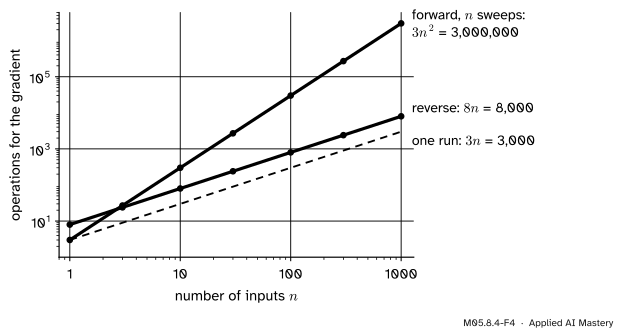
n = 1000: run  3000 ops | forward 3,000,000 ops,  0.8647 s | reverse  8,000 ops,  0.0035 s

M05.8.4-F4

The counts printed by the code. Reverse mode stays a fixed multiple of one run; forward mode grows like \(n\) runs.

The counts are exact and do not depend on the machine: \({3n}\) for a run, \({3n^2}\) for \(n\) forward sweeps, and \({8n}\) for reverse mode (the \({3n}\) forward operations, then one multiply-add for each of the \({5n}\) edges). The times are printed, not checked, because they do depend on the machine; the pattern is the same everywhere. At \({n = 1}\) forward mode is cheaper, 3 operations against 8; by \({n = 1000}\) it does 375 times the work.

Last, forward over reverse. The backward sweep of the running program, written out as plain code (the steps of M05.8.3), is itself a program, so it can run on dual numbers:

def gradient(x1, x2):
    """Reverse mode for ln x1 + x1 x2 - sin x2, written out: a forward pass, then the adjoints."""
    v1, v2, v3 = ln(x1), x1 * x2, sin(x2)               # the forward pass (v4, v5 are not needed)
    d5 = 1.0
    d4, d3 = d5, -d5
    d1, d2 = d4, d4
    d0 = d3 * cos(x2)
    dm1 = d2 * x2
    d0 = d0 + d2 * x1
    dm1 = dm1 + d1 / x1
    return dm1, d0

g = gradient(2.0, 5.0)
print("gradient:", [round(float(v), 3) for v in g])
for v in ((1.0, 0.0), (0.0, 1.0)):
    out = gradient(Dual(2.0, v[0]), Dual(5.0, v[1]))
    print(f"H v for v = {v}:", [round(o.tangent, 3) for o in out])

gradient: [5.5, 1.716]
H v for v = (1.0, 0.0): [-0.25, 1.0]
H v for v = (0.0, 1.0): [1.0, -0.959]

The two products are the columns of the Hessian \({\begin{pmatrix} -1/x_1^2 & 1 \\ 1 & \sin x_2 \end{pmatrix}}\) at \({(2, 5)}\): \({(-0.25,\ 1)}\) and \({(1,\ -0.959)}\). In JAX the same idea is jax.jvp applied to jax.grad(f).

Explore

The graph stepper in lesson M05.8.3 keeps count. Run the full gradient both ways at any point: forward mode needs two sweeps (one per input), reverse mode one (one per output), and the read-out sets both against the four runs of \(f\) that central differences would need. With two inputs and one output the saving is small; the counts in this lesson show how it grows with the number of inputs.

Pitfalls

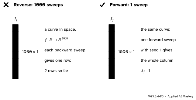
M05.8.4-F5

Wrong beside right. For one input and many outputs, reverse mode needs a sweep per output; forward mode fills the whole column in one.

“Reverse mode is always faster.”

It is faster when there are many more inputs than outputs, which is the case for a loss. For a Jacobian that is tall, with few inputs and many outputs, forward mode needs fewer sweeps, and for small or square problems its simplicity often wins outright. Count both before choosing.

“Reverse mode costs nothing extra.”

Its arithmetic is a small multiple of one run, but it stores the whole forward trace. A deep network trained with a large batch can run out of memory long before it runs out of time, which is why checkpointing exists (M05.9.4). Forward mode keeps only the current values and tangents.

“A Hessian-vector product needs the Hessian.”

It needs only a forward sweep through the gradient program. Forming the \({n \times n}\) Hessian of a model with a million weights would need \({10^{12}}\) numbers; \({\mat{H}\vect{v}}\) needs a few gradients’ worth of work and memory.

Check yourself

Recall

1. Which order of multiplying \({\mat{J}_f = \mat{A}\mat{B}\mat{C}}\) does each mode use?

Show answer

Forward mode multiplies right to left, starting from seed vectors at the input; reverse mode multiplies left to right, starting from a row of adjoints at the output.

2. How many sweeps does each mode need for the full Jacobian of \({f : \R^n \to \R^m}\)?

Show answer

Forward mode \(n\), one column per sweep; reverse mode \(m\), one row per sweep.

3. How many multiplications does \({(\mat{A}\mat{B})\mat{C}}\) take for shapes \({1 \times 100}\), \({100 \times 100}\), \({100 \times 1000}\)?

Show answer

\({10{,}000 + 100{,}000 = 110{,}000}\), against \({10{,}100{,}000}\) for \({\mat{A}(\mat{B}\mat{C})}\).

4. Why does reverse mode need memory that forward mode does not?

Show answer

Its first factor is the Jacobian of the last stage, which depends on values that exist only after a full forward pass, so every value the local derivatives need is stored on the tape.

5. How is \({\mat{H}\vect{v}}\) computed without forming \(\mat{H}\)?

Show answer

Run the reverse-mode gradient program on dual numbers \({\vect{x} + \vect{v}\varepsilon}\); the \(\varepsilon\) parts are \({\tfrac{d}{d\alpha}\nabla f(\vect{x} + \alpha\vect{v}) = \mat{H}\vect{v}}\).

Exercises

1. ★ A function \({f : \R^5 \to \R^{10}}\) has the Jacobian chain \({\mat{J}_f = \mat{A}\mat{B}\mat{C}}\) with shapes \({10 \times 50}\), \({50 \times 50}\) and \({50 \times 5}\). Count the multiplications of both orders. Which mode is cheaper, and does that agree with the rule of thumb?

Show solution

Left to right: \({10 \cdot 50 \cdot 50 = 25{,}000}\), then \({10 \cdot 50 \cdot 5 = 2{,}500}\), total 27,500. Right to left: \({50 \cdot 50 \cdot 5 = 12{,}500}\), then \({10 \cdot 50 \cdot 5 = 2{,}500}\), total 15,000. Right to left, forward mode, is cheaper, as the rule of thumb says, since there are fewer inputs (5) than outputs (10).

2. ★★ A network maps a 784-pixel image to 10 class scores and has 100,000 weights. How many sweeps of each mode give (a) the Jacobian of the 10 scores with respect to the 784 pixels, and (b) the gradient of the loss with respect to the weights?

Show solution

(a) The Jacobian is \({10 \times 784}\): forward mode needs 784 sweeps, reverse mode 10. Reverse wins. (b) The loss is one number and the weights are 100,000 inputs: reverse mode needs one sweep, forward mode 100,000. This second case is training, and the reason backpropagation is reverse mode.

3. ★★★ Let \({\mat{J} = \vect{u}\T\mat{M}_1\mat{M}_2 \cdots \mat{M}_k}\) with \({\vect{u} \in \R^p}\) and every \(\mat{M}_i\) of size \({p \times p}\). Show that left to right costs \({k\,p^2}\) multiplications and right to left \({(k - 1)\,p^3 + p^2}\). Evaluate both for \({p = 100}\), \({k = 3}\).

Show solution

Left to right: every partial product is a row \({1 \times p}\), and a row times a \({p \times p}\) matrix costs \({1 \cdot p \cdot p = p^2}\); there are \(k\) such steps, so \({k\,p^2}\). Right to left: the \({k - 1}\) products of two \({p \times p}\) matrices cost \(p^3\) each, and the final row times the \({p \times p}\) result costs \(p^2\), so \({(k - 1)\,p^3 + p^2}\). For \({p = 100}\) and \({k = 3}\): \({30{,}000}\) against \({2{,}010{,}000}\), about 67 times as much. With \(p\) growing, it is \(p^2\) against \(p^3\), the example Bright, Edelman and Johnson give in section 2.5.

Summary card

Same derivatives, different order: count inputs and outputs.

The anchor figure again: the chain A, B, C of shapes 1 by 100, 100 by 100 and 100 by 1000, multiplied left to right for 110,000 multiplications and right to left for 10,100,000. — M05.8.4-F1
Left to right with a row is cheap.

Forward mode: right to left, a column per sweep, \(n\) sweeps.
Reverse mode: left to right, a row per sweep, \(m\) sweeps, and a stored tape.
A gradient by reverse mode costs a small constant times one run, for any \(n\).
\({\mat{H}\vect{v} = \tfrac{d}{d\alpha}\nabla f(\vect{x} + \alpha\vect{v})}\): forward over reverse.

Sources and next steps

Sources. Each was opened and checked against this lesson on 15 November 2026.

A. G. Baydin, B. A. Pearlmutter, A. A. Radul and J. M. Siskind, Automatic Differentiation in Machine Learning: a Survey, JMLR 18(153), 2018. Section 3.1: forward mode builds the Jacobian one column per evaluation, \(n\) in all; section 3.2: reverse mode costs \({m\,c\,\text{ops}(f)}\) against \({n\,c\,\text{ops}(f)}\), with \({c < 6}\) and typically 2 to 3 (after Griewank and Walther), and needs storage growing with the number of operations, eased by checkpointing; section 4.1: Hessian-vector products in \({O(n)}\) by combining the two modes.
P. Bright, A. Edelman and S. G. Johnson, Matrix Calculus (for Machine Learning and Beyond): section 2.5 names left-to-right multiplication of the Jacobian chain reverse mode and right-to-left forward mode, counts \(mp\) dot products of length \(q\) for an \({m \times q}\) times \({q \times p}\) product (2.5.1) and gives the \(n^2\) against \(n^3\) example (Example 16); section 8.4 compares the modes, including the tape and the remark that forward mode can win until \(n\) is fairly large; section 8.4.1 derives forward-over-reverse Hessian-vector products.
M. P. Deisenroth, A. A. Faisal and C. S. Ong, Mathematics for Machine Learning, section 5.6.2, equations (5.119) to (5.121): forward and reverse mode differ in the order of multiplying the chain of derivatives, and reverse mode is cheaper when the inputs outnumber the outputs.

Next. Module M05.9 runs reverse mode on a small neural network and recognises it as backpropagation. The engineering of real engines is DL01.6 and P08.6.

This lesson unlocks

M05.9 Backpropagation as reverse-mode differentiation DL01.6 Build an autodiff engine from scratch P08.6 Automatic differentiation engines (planned)

Your progress is saved in this browser only. No account, no tracking.