Derive with differentials the change of an inverse, -X^(-1) dX X^(-1), and of a determinant, det X tr(X^(-1) dX), so that the gradient of log det X is X^(-T). Then use them to find the maximum-likelihood covariance of a Gaussian.
M05.7.4L2 Intermediate25 minIn review (what this means)
The maths and code on this page are checked by automated tests on every change, but an independent reader has not signed it off yet. Spot a mistake or a confusing step? Tell us.
Derive d(X^(-1)) = -X^(-1) dX X^(-1) from X X^(-1) = I.
Explain with a picture why det(I + E) is about 1 + tr(E), and derive d det X = det X tr(X^(-1) dX).
State and use the gradient of log det X, X^(-T), and its symmetric case X^(-1).
Derive that the maximum-likelihood covariance of a Gaussian is the sample covariance with the factor 1/n.
The question
The log-likelihood of data under a Gaussian contains the term \({-\tfrac{n}{2}\ln\det\mat{\Sigma}}\) and the inverse \(\mat{\Sigma}^{-1}\). To fit the covariance \(\mat{\Sigma}\) by maximum likelihood, or to train a normalising flow, which needs \(\ln\abs{\det\mat{J}}\), you must differentiate a determinant and an inverse with respect to a matrix. What are those derivatives, and why does a transpose appear in the gradient of \(\ln\det\mat{X}\)?
From the last lesson
1. For \(\mat{Y} = \mat{X}\mat{W} + \vect{1}\vect{b}\T\) and \(\mat{G} = \partial L/\partial\mat{Y}\), what is \(\nabla_{\mat{W}} L\)?
Show answer
\(\mat{X}\T\mat{G}\), with the shape of \(\mat{W}\).
2. What is the gradient of cross-entropy after softmax with respect to the scores?
Show answer
\(\vect{p} - \vect{y}\), and \((\mat{P} - \mat{T})/B\) for the mean over a batch.
Intuition
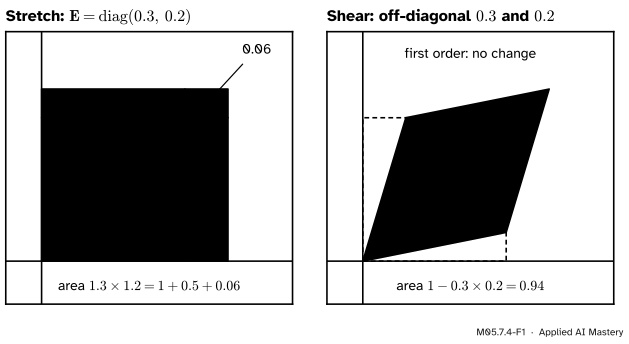
The determinant measures how a matrix scales area (M02.8). So ask a geometric question: how does the area of the unit square change under \({\mat{I} + \mat{E}}\), when \(\mat{E}\) is small?
M05.7.4-F1
The unit square under \({\mat{I} + \mat{E}}\). Diagonal entries of \(\mat{E}\) stretch the sides and add area \({e_{11} + e_{22}} = \operatorname{tr}(\mat{E})\), plus a corner that is a product of two small numbers. Off-diagonal entries shear the square; the area changes only by a product of two small numbers.
To first order, then, only the diagonal of \(\mat{E}\) matters, and it adds up to the trace: \({\det(\mat{I} + \mat{E})} \approx {1 + \operatorname{tr}(\mat{E})}\). Every result in this lesson grows from that picture and from one more fact: \({\mat{X}\mat{X}^{-1}} = \mat{I}\) never changes.
Build it up
Step 1. The 2 by 2 case exactly. For \({\mat{I} + \mat{E}}\) with entries \(1 + e_{11}\), \(e_{12}\), \(e_{21}\) and \(1 + e_{22}\),
The bracket is a sum of products of two entries of \(\mat{E}\): second order. The figure’s numbers are \({1 + 0.5 + 0.06}\) and \({1 + 0 - 0.06}\).
Step 2. Move the nudge to the identity. For an invertible \(\mat{X}\), factor it out: \({\mat{X} + d\mat{X}} = {\mat{X}(\mat{I} + \mat{X}^{-1}d\mat{X})}\). Determinants multiply, so
so \(\nabla\det\mat{X} = \det\mat{X}\;\mat{X}^{-\top}\) and \(\nabla\ln\det\mat{X} = \mat{X}^{-\top}\), where \(\mat{X}^{-\top}\) is the transpose of the inverse. For symmetric \(\mat{X}\) the gradient of \(\ln\det\mat{X}\) is \(\mat{X}^{-1}\).
The inverse. The product \({\mat{X}\mat{X}^{-1}} = \mat{I}\) is constant, so its differential is zero. The product rule of M05.7.2 gives
Move the first term across and multiply on the left by \(\mat{X}^{-1}\): \({d(\mat{X}^{-1})} = {-\mat{X}^{-1}d\mat{X}\,\mat{X}^{-1}}\). For a \({1 \times 1}\) matrix this is the familiar \(d(1/x) = -dx/x^2\); for matrices the two factors of \(\mat{X}^{-1}\) must stay on either side of \(d\mat{X}\).
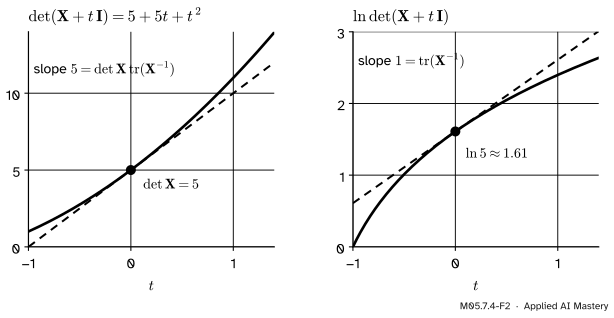
The determinant. Step 2 is the derivation of the second line; it rests on \({\det(\mat{I} + \mat{E})} = {1 + \operatorname{tr}(\mat{E})}\) plus second-order terms, which Step 1 showed for 2 by 2 matrices and the box below proves for any size. To read off the gradient, write \({\det\mat{X}\,\operatorname{tr}(\mat{X}^{-1}d\mat{X})} = {\operatorname{tr}(\mat{G}\T d\mat{X})}\) with \(\mat{G}\T = \det\mat{X}\,\mat{X}^{-1}\), so \({\mat{G}} = {\det\mat{X}\,\mat{X}^{-\top}}\).
The log-determinant. By the chain rule for one variable, \({d\ln u} = {du/u}\), so dividing the second line by \(\det\mat{X}\) gives the third. Its gradient is \(\mat{X}^{-\top}\). If \(\det\mat{X}\) is negative, \(\ln\abs{\det\mat{X}} = \ln(-\det\mat{X})\) has the same differential \(du/u\), so the gradient of \(\ln\abs{\det\mat{X}}\) is \(\mat{X}^{-\top}\) for every invertible \(\mat{X}\).
Go deeper: det(I + E) = 1 + tr(E) + second order, for any size
Write the determinant as Leibniz’s sum over permutations \(\pi\) of \(\{1, \dots, n\}\): \({\det\mat{M}} = {\sum_\pi \operatorname{sgn}(\pi)\, m_{1\pi(1)} \cdots m_{n\pi(n)}}\). For \(\mat{M} = \mat{I} + \mat{E}\), an entry off the diagonal is \(e_{ij}\), which is small. A permutation other than the identity moves at least two indices, so its product contains at least two off-diagonal factors and is second order. The identity permutation gives \({(1 + e_{11})(1 + e_{22}) \cdots (1 + e_{nn})}\), which is \({1 + e_{11} + \dots + e_{nn}}\) plus products of two or more \(e_{ii}\). So \({\det(\mat{I} + \mat{E})} = {1 + \operatorname{tr}(\mat{E})}\) plus second-order terms.
Use 1: the maximum-likelihood covariance. Data \(\vect{x}_1, \dots, \vect{x}_n\) in \(\R^d\) are modelled as Gaussian with mean \(\vect{\mu}\) and covariance \(\mat{\Sigma}\) (the Gaussian in full is M07.3; here only its formula is needed). Take \(\vect{\mu}\) as the sample mean, which is its maximum-likelihood value whatever \(\mat{\Sigma}\) is, and write \(\vect{d}_i = \vect{x}_i - \vect{\mu}\) for the deviation of point \(i\). The log-likelihood is
Each quadratic term is a number, equal to its trace, and cyclic order turns it into \({\operatorname{tr}(\mat{\Sigma}^{-1}\vect{d}_i\vect{d}_i\T)}\). Adding over \(i\) gives \({n\operatorname{tr}(\mat{\Sigma}^{-1}\mat{S})}\) with the sample covariance\({\mat{S}} = {\tfrac{1}{n}\sum_i \vect{d}_i\vect{d}_i\T}\). So
where \({\mat{M}} = {\mat{\Sigma}^{-1} - \mat{\Sigma}^{-1}\mat{S}\mat{\Sigma}^{-1}}\).
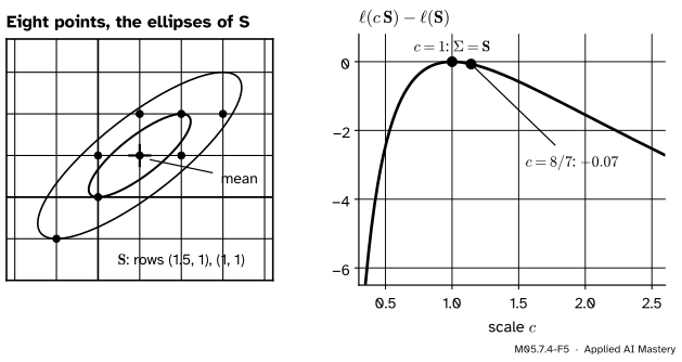
The second line uses \(d(\mat{\Sigma}^{-1})\) from the theorem; the last moves \(\mat{\Sigma}^{-1}\mat{S}\) to the front cyclically. The change is zero for every \(d\mat{\Sigma}\) only when \({\mat{\Sigma}^{-1}} = {\mat{\Sigma}^{-1}\mat{S}\mat{\Sigma}^{-1}}\). Multiplying by \(\mat{\Sigma}\) on the left and on the right gives \(\mat{\Sigma} = \mat{S}\). This is the only point where the change is zero, and (for an invertible \(\mat{S}\)) the log-likelihood falls towards \(-\infty\) both as \(\mat{\Sigma}\) approaches a singular matrix and as it grows without bound, so this point is the maximum. The maximum-likelihood covariance is the sample covariance with the factor \(1/n\), not \(1/(n - 1)\). As in Bishop’s derivation, the symmetry of \(\mat{\Sigma}\) was not imposed, and the answer comes out symmetric anyway.
M05.7.4-F5
The covariance found by maximum likelihood, for eight invented points. Scaling the guess away from \(\mat{S}\) in either direction lowers the log-likelihood; the unbiased estimate, \(8/7\) times \(\mat{S}\), is slightly lower.
Use 2: normalising flows. A flow pushes simple noise \(\vect{x}\) through an invertible map to \(\vect{y}\). For a linear flow \(\vect{y} = \mat{W}\vect{x}\) the change-of-variables rule of M05.6.4 gives \({\ln p_Y(\vect{y})} = {\ln p_X(\mat{W}^{-1}\vect{y}) - \ln\abs{\det\mat{W}}}\). Training maximises this over \(\mat{W}\), so it needs the gradient of \(\ln\abs{\det\mat{W}}\), which is \(\mat{W}^{-\top}\). Computing an inverse costs about \(d^3\) operations, which is why practical flows (DL06.7) use maps whose Jacobian is triangular: then the determinant is the product of the diagonal and its logarithm a sum.
Worked example
A symmetric matrix. Take \(\mat{X}\) with rows \((3, 1)\) and \((1, 2)\). Then \({\det\mat{X}} = {3 \cdot 2 - 1 \cdot 1} = 5\) and, by the 2 by 2 formula, \({\mat{X}^{-1}} = {\tfrac{1}{5}[[2, -1], [-1, 3]]}\), with rows \((0.4, -0.2)\) and \((-0.2, 0.6)\).
M05.7.4-F3
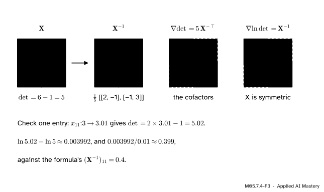
The worked example: the inverse, the two gradients, and one entry checked by a nudge.
The gradient of the determinant is \({5\,\mat{X}^{-\top}}\), with rows \((2, -1)\) and \((-1, 3)\). Check it directly: \({\det\mat{X}} = {x_{11}x_{22} - x_{12}x_{21}}\), so \(\pd{\det}{x_{11}} = x_{22} = 2\), \(\pd{\det}{x_{12}} = -x_{21} = -1\), \(\pd{\det}{x_{21}} = -x_{12} = -1\) and \(\pd{\det}{x_{22}} = x_{11} = 3\). These are the cofactors of \(\mat{X}\).
The gradient of \({\ln\det\mat{X}}\) is \(\mat{X}^{-1}\) itself, because \(\mat{X}\) is symmetric. Nudge \(x_{11}\) from 3 to 3.01: the determinant becomes \({2 \cdot 3.01 - 1} = 5.02\), and
against the predicted slope \((\mat{X}^{-1})_{11} = 0.4\).
The inverse under the same nudge. With \({d\mat{X} = 0.01\,\mat{E}_{11}}\) the theorem predicts \({-0.01\,\mat{X}^{-1}\mat{E}_{11}\mat{X}^{-1}}\). The product \(\mat{X}^{-1}\mat{E}_{11}\mat{X}^{-1}\) is column 1 of \(\mat{X}^{-1}\) times row 1, the outer product of \((0.4, -0.2)\) with itself:
The exact change, \({\tfrac{1}{5.02}[[2, -1], [-1, 3.01]]} - \mat{X}^{-1}\), has first row about \((-0.00159, 0.00080)\), against the prediction \((-0.0016, 0.0008)\).
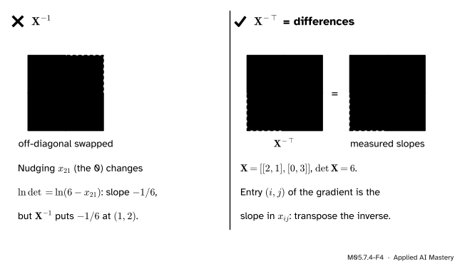
A non-symmetric matrix. For \(\mat{X}\) with rows \((2, 1)\) and \((0, 3)\), \(\det\mat{X} = 6\) and \(\mat{X}^{-1}\) has rows \((1/2, -1/6)\) and \((0, 1/3)\). The gradient of \(\ln\det\mat{X}\) is its transpose, with rows \((1/2, 0)\) and \((-1/6, 1/3)\). Directly: \({\det\mat{X}} = {x_{11}x_{22} - x_{12}x_{21}}\), so \(\pd{\ln\det}{x_{21}} = -x_{12}/6 = -1/6\) and \(\pd{\ln\det}{x_{12}} = -x_{21}/6 = 0\). The transpose matters.
Code
From scratch: each identity against central differences, entry by entry.
import numpy as npdef num_grad(f, X, h=1e-6): G = np.zeros_like(X)for index in np.ndindex(X.shape): E = np.zeros_like(X) E[index] = h G[index] = (f(X + E) - f(X - E)) / (2* h)return Grng = np.random.default_rng(11)X = rng.normal(size=(4, 4)) +4* np.eye(4) # invertible, not symmetricinv = np.linalg.inv(X)gaps = {"det": np.abs(num_grad(np.linalg.det, X) - np.linalg.det(X) * inv.T).max() /abs(np.linalg.det(X)),"ln det": np.abs(num_grad(lambda M: np.log(np.linalg.det(M)), X) - inv.T).max(),}dX =1e-6* rng.normal(size=(4, 4))exact = np.linalg.inv(X + dX) - invgaps["inverse"] = np.abs(exact - (-inv @ dX @ inv)).max() / np.abs(exact).max()for name, gap in gaps.items():print(f"{name:8s} relative gap {gap:.1e}")Xs = np.array([[3.0, 1.0], [1.0, 2.0]])print("det =", np.linalg.det(Xs).round(12), " inverse =", np.linalg.inv(Xs).round(12).tolist())print("grad det =", (np.linalg.det(Xs) * np.linalg.inv(Xs).T).round(12).tolist())print("nudge slope:", (np.log(np.linalg.det(Xs + np.diag([0.01, 0]))) - np.log(5)) /0.01)Xt = np.array([[2.0, 1.0], [0.0, 3.0]])print("non-symmetric: grad ln det =", num_grad(lambda M: np.log(np.linalg.det(M)), Xt).round(6).tolist())
det      relative gap 5.9e-10
ln det   relative gap 6.0e-10
inverse  relative gap 3.9e-07
det = 5.0   inverse = [[0.4, -0.2], [-0.2, 0.6]]
grad det = [[2.0, -1.0], [-1.0, 3.0]]
nudge slope: 0.399202126953746
non-symmetric: grad ln det = [[0.5, 0.0], [-0.166667, 0.333333]]
NumPy’s numpy.linalg.slogdet returns the sign and the logarithm of the absolute value of the determinant without forming the determinant itself, which can overflow or underflow. It works for a negative determinant too, where the gradient of \(\ln\abs{\det\mat{X}}\) is still \(\mat{X}^{-\top}\):
sign -1.0  log|det| 1.609438  gap from X^-T: 1.2e-10
det(0.1 I_500) = 0.0   slogdet: SlogdetResult(sign=np.float64(1.0), logabsdet=np.float64(-1151.2925464970251))
Finally the Gaussian: the eight points of the figure, the sample covariance with \(1/n\), a check that the gradient of the log-likelihood vanishes there, and SciPy’s log-density as the library version.
mean [1. 1.]   S = [[1.5, 1.0], [1.0, 1.0]]   np.cov(bias=True): [[1.5, 1.0], [1.0, 1.0]]
log-likelihood at S: -19.9304   SciPy: -19.9304
largest gradient entry at S: 1.8e-09
at 8/7 S, relative to S: -0.0683
Explore
The gradient heatmap of M05.7.2 has a preset for \(\ln\det\mat{X}\). Make \(\mat{X}\) non-symmetric and switch to the common mistake, \(\mat{X}^{-1}\): the two off-diagonal cells disagree with the measured slopes. Move \(\mat{X}\) towards a singular matrix and watch the gradient grow without bound.
Pitfalls
M05.7.4-F4
Wrong beside right for the gradient of \(\ln\det\mat{X}\) with a non-symmetric \(\mat{X}\): the inverse puts the two off-diagonal slopes in each other’s places.
“The gradient of \(\ln\det\mat{X}\) is \(\mat{X}^{-1}\).”
Only for symmetric \(\mat{X}\). In general it is \(\mat{X}^{-\top}\), as the figure shows. Covariance matrices are symmetric, so formulas copied from statistics often omit the transpose; a flow’s weight matrix is not symmetric, and there it matters.
“\(d(\mat{X}^{-1}) = -\mat{X}^{-2}\,d\mat{X}\), as for numbers.”
Matrices do not commute, so \(d\mat{X}\) cannot be moved past \(\mat{X}^{-1}\). The correct form, \({-\mat{X}^{-1}d\mat{X}\,\mat{X}^{-1}}\), keeps one factor on each side. The two agree only when \(d\mat{X}\) commutes with \(\mat{X}\), for example when both are diagonal.
“To get \(\ln\det\), take the log of det.”
The determinant of a large matrix overflows or underflows long before its logarithm does: the determinant of \(0.1\,\mat{I}\) of size 500 is \(10^{-500}\), which NumPy returns as 0, so the log is \(-\infty\). Use numpy.linalg.slogdet, which returns \(500 \ln 0.1 \approx -1151.3\) directly.
“The Matrix Cookbook says the gradient for symmetric \(\mat{X}\) is \(2\mat{X}^{-1} - (\mat{X}^{-1} \circ \mat{I})\).”
That formula treats \(x_{ij}\) and \(x_{ji}\) as one variable, so a nudge moves two entries at once, and the off-diagonal slopes double. It answers a different question. This course differentiates with respect to every entry separately, which gives \(\mat{X}^{-1}\); the derivation of \(\mat{\Sigma} = \mat{S}\) above is valid either way, because a matrix that makes \(d\ell\) zero for every nudge also makes it zero for symmetric nudges.
Check yourself
Recall
1. What is \(d(\mat{X}^{-1})\), and from which identity does it come?
Show answer
\({-\mat{X}^{-1}d\mat{X}\,\mat{X}^{-1}}\), from differentiating \({\mat{X}\mat{X}^{-1}} = \mat{I}\) with the product rule.
2. To first order, what is \(\det(\mat{I} + \mat{E})\)?
Show answer
\(1 + \operatorname{tr}(\mat{E})\).
3. What is the gradient of \(\ln\det\mat{X}\), and when is it \(\mat{X}^{-1}\)?
Show answer
\(\mat{X}^{-\top}\); it equals \(\mat{X}^{-1}\) when \(\mat{X}\) is symmetric.
4. What is the gradient of \(\det\mat{X}\)?
Show answer
\(\det\mat{X}\;\mat{X}^{-\top}\), the matrix of cofactors.
5. What is the maximum-likelihood covariance of a Gaussian?
Show answer
The sample covariance with the factor \(1/n\): \({\tfrac{1}{n}\sum_i (\vect{x}_i - \vect{\mu})(\vect{x}_i - \vect{\mu})\T}\), with \(\vect{\mu}\) the sample mean.
Exercises
1.★ For \(\mat{X}\) with rows \((4, 2)\) and \((1, 1)\), find \(\det\mat{X}\) and the gradient of \(\ln\det\mat{X}\), and check one entry directly.
Show solution
\(\det\mat{X} = 4 - 2 = 2\) and \(\mat{X}^{-1} = \tfrac{1}{2}[[1, -2], [-1, 4]]\), so the gradient is \(\mat{X}^{-\top} = \tfrac{1}{2}[[1, -1], [-2, 4]]\), with rows \((0.5, -0.5)\) and \((-1, 2)\). Directly, \(\ln\det = \ln(x_{11}x_{22} - x_{12}x_{21})\), so \(\pd{}{x_{21}} = -x_{12}/2 = -1\): entry \((2, 1)\).
2.★★ Show that the gradient of \(f(\mat{X}) = \vect{a}\T\mat{X}^{-1}\vect{b}\) is \({-\mat{X}^{-\top}\vect{a}\vect{b}\T\mat{X}^{-\top}}\).
Show solution
\(df = \vect{a}\T d(\mat{X}^{-1})\vect{b} = -\vect{a}\T\mat{X}^{-1}d\mat{X}\,\mat{X}^{-1}\vect{b}\). It is a number, so take the trace and move \(\mat{X}^{-1}\vect{b}\) to the front:
So \(\mat{G}\T = -\mat{X}^{-1}\vect{b}\vect{a}\T\mat{X}^{-1}\) and \({\mat{G}} = {-\mat{X}^{-\top}\vect{a}\vect{b}\T\mat{X}^{-\top}}\), which is (5.103) of MML.
3.★★★ Write the log-likelihood in terms of the precision\(\mat{\Lambda} = \mat{\Sigma}^{-1}\), as \({\text{const} + \tfrac{n}{2}\big(\ln\det\mat{\Lambda} - \operatorname{tr}(\mat{\Lambda}\mat{S})\big)}\), and find its maximiser. Why is this easier?
Show solution
\(\ln\det\mat{\Sigma} = -\ln\det\mat{\Lambda}\) because \(\det(\mat{\Lambda}^{-1}) = 1/\det\mat{\Lambda}\), and \(\operatorname{tr}(\mat{\Sigma}^{-1}\mat{S}) = \operatorname{tr}(\mat{\Lambda}\mat{S})\), which gives the form shown. Its differential is \({\tfrac{n}{2}\big(\operatorname{tr}(\mat{\Lambda}^{-1}d\mat{\Lambda}) - \operatorname{tr}(\mat{S}\,d\mat{\Lambda})\big)}\), so the gradient is \({\tfrac{n}{2}(\mat{\Lambda}^{-\top} - \mat{S}\T)}\), zero when \(\mat{\Lambda}^{-1} = \mat{S}\), that is \(\mat{\Sigma} = \mat{S}\) again. It is easier because the trace term is linear in \(\mat{\Lambda}\), so no inverse has to be differentiated.
Log-determinant:\(\nabla\ln\abs{\det\mat{X}} = \mat{X}^{-\top}\), and \(\mat{X}^{-1}\) when symmetric.
Gaussian: the maximum-likelihood \(\mat{\Sigma}\) is \(\mat{S}\), with factor \(1/n\).
Sources and next steps
Sources. Each was opened and checked against this lesson on 15 November 2026.
Paige Bright, Alan Edelman and Steven G. Johnson, Matrix Calculus (for Machine Learning and Beyond), course notes of MIT 18.S096: Example 19 in Section 2.6 (\(d(\mat{A}^{-1}) = -\mat{A}^{-1}d\mat{A}\,\mat{A}^{-1}\) from the product rule); Theorem 39 in Section 7.1 (\(\nabla\det\mat{A} = \det\mat{A}\,\mat{A}^{-\top}\), the cofactor matrix, with a proof through \({\det(\mat{I} + d\mat{A}) - 1} = {\operatorname{tr}(d\mat{A})}\)); Section 7.2.2 (the logarithmic derivative \(\operatorname{tr}(\mat{A}^{-1}d\mat{A})\)).
Kaare Brandt Petersen and Michael Syskind Pedersen, The Matrix Cookbook, version of 15 November 2012: (40), (42) and (43) in Section 2; (49) and (57) in Section 2.1; and (141) in Section 2.8.2 for symmetric matrices treated as structured.
Christopher M. Bishop, Pattern Recognition and Machine Learning, Section 2.3.4: the maximum-likelihood covariance (2.122) with factor \(1/N\), found by ignoring the symmetry constraint, and its bias (2.124).
NumPy reference, numpy.linalg.slogdet: the sign and the log of the absolute determinant, robust to overflow and underflow, with the example of \(0.1\,\mat{I}\) of size 500.
Next. M05.8, Computational graphs and automatic differentiation, lets a program apply rules like these automatically, one elementary operation at a time.