Gradients of a dense layer and of softmax with cross-entropy
Derive with differentials the three gradients of a dense layer, X-transpose G, G W-transpose and the column sums of G, then the softmax Jacobian and the famous p minus y, and check every shape on a batch of two examples.
M05.7.3L2 Intermediate25 minIn review (what this means)
The maths and code on this page are checked by automated tests on every change, but an independent reader has not signed it off yet. Spot a mistake or a confusing step? Tell us.
Derive the gradients of a batch dense layer with respect to its weights, its inputs and its bias, given the gradient with respect to its outputs.
Derive the softmax Jacobian diag(p) - p p-transpose and the gradient p - y of cross-entropy after softmax.
Pass a gradient through an elementwise activation as an elementwise product.
Compute every gradient of a small layer by hand and check it, with its shape, against finite differences.
The question
A dense layer takes a batch of 64 images of 784 pixels to 100 outputs. Its weight matrix has 78,400 entries and its output has 6,400. The full Jacobian of the output with respect to the weights would have \({6{,}400 \times 78{,}400}\), about 502 million, entries. Every deep-learning library computes the weight gradient of this layer in a fraction of a millisecond. What does it compute instead?
From the last lesson
1. If \(df = \operatorname{tr}(\mat{G}\T d\mat{X})\) for every \(d\mat{X}\), what is \(\nabla_{\mat{X}} f\)?
Show answer
\(\mat{G}\).
2. What is the gradient of \(\vect{a}\T\mat{X}\vect{b}\)?
Show answer
\(\vect{a}\vect{b}\T\), which has the shape of \(\mat{X}\).
Intuition
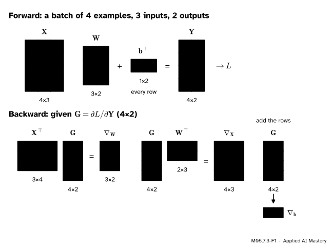
Think of the loss as a machine downstream of the layer. Whatever it is, it hands back one number for each output of the layer: the matrix \(\mat{G}\) of how much the loss changes per unit change of each output. The layer’s job in the backward pass is to turn \(\mat{G}\) into gradients for its weights, its bias and its input. Each turns out to be a single product, and the shapes leave only one possible way to write it.
M05.7.3-F1
The dense layer and its three gradients, drawn by shape. \(\mat{X}\T\mat{G}\) is the only product of the available pieces with the shape of \(\mat{W}\), \(\mat{G}\mat{W}\T\) the only one with the shape of \(\mat{X}\), and adding the rows of \(\mat{G}\) gives the shape of \(\vect{b}\).
So the library never builds the 502-million-entry Jacobian. It multiplies \(\mat{X}\T\) (784 by 64) by \(\mat{G}\) (64 by 100): about five million multiply-adds, and the answer has exactly the shape of the weights.
Build it up
Step 1. The layer. Each row of \(\mat{X}\) is one example, \(\vect{x}_k\T\), with \(d\) features. The layer computes
where \(\mat{W}\) is \({d \times m}\), \(\vect{b}\) is in \(\R^m\) and \(\vect{1}\) is a column of \(B\) ones, so \(\vect{1}\vect{b}\T\) copies \(\vect{b}\T\) into every row. Row \(k\) of \(\mat{Y}\) is \({\vect{x}_k\T\mat{W} + \vect{b}\T}\), the outputs for example \(k\).
Step 2. What arrives from the loss. Write \(\mat{G} = \partial L / \partial \mat{Y}\) for the gradient of the loss with respect to the outputs, a \({B \times m}\) matrix. By the differential method of M05.7.2 this means \(dL = {\operatorname{tr}(\mat{G}\T d\mat{Y})}\).
Step 3. One example at a time. For a single example, \(\vect{y}\T = \vect{x}\T\mat{W} + \vect{b}\T\) and the loss sends back a row \(\vect{g}\T\). Output \(j\) is \({\sum_i x_i w_{ij}}\), so weight \(w_{ij}\) affects only output \(j\), at the rate \(x_i\). Hence \(\pd{L}{w_{ij}} = x_i\, g_j\): the gradient is the outer product \(\vect{x}\vect{g}\T\).
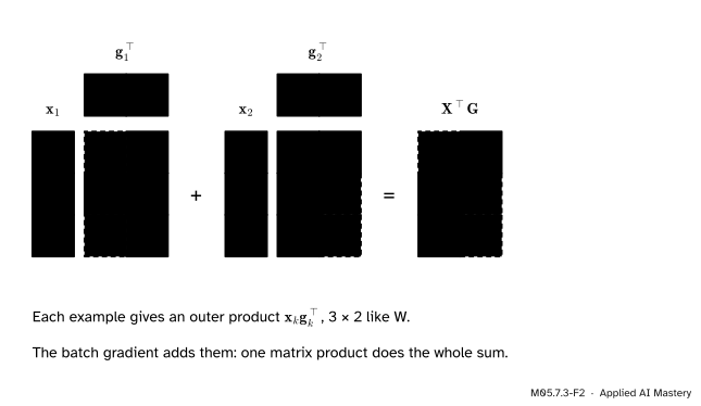
Step 4. A batch adds up. The loss of a batch is a sum over examples (or a mean, with its factor inside \(\mat{G}\)), so the weight gradient is a sum of outer products, one per example. The sum of \(\vect{x}_k\vect{g}_k\T\) over \(k\) is exactly the matrix product \(\mat{X}\T\mat{G}\).
M05.7.3-F2
The weight gradient of the worked example below as a sum of two outer products. Each is a small multiplication table: inputs down the side, output gradients across the top.
The formal statement
NoteTheorem: the gradients of a dense layer
For \(\mat{Y} = \mat{X}\mat{W} + \vect{1}\vect{b}\T\) and a loss \(L\) with \(\mat{G} = \partial L / \partial \mat{Y}\),
\[
\begin{aligned}
\nabla_{\mat{W}} L &= \mat{X}\T\mat{G} && (d \times m), \\
\nabla_{\mat{X}} L &= \mat{G}\mat{W}\T && (B \times d), \\
\nabla_{\vect{b}} L &= \mat{G}\T\vect{1} && (m \times 1),
\end{aligned}
\]
the last being the column sums of \(\mat{G}\).
Derivation. The rules of M05.7.2 give \(d\mat{Y} = {d\mat{X}\,\mat{W}} + {\mat{X}\,d\mat{W}} + {\vect{1}\,d\vect{b}\T}\), so \(dL\) has three terms, one per variable. Each is rearranged into the form \({\operatorname{tr}(\text{gradient}\T\,d\text{variable})}\):
The first line uses \({(\mat{X}\T\mat{G})\T} = {\mat{G}\T\mat{X}}\). The second moves \(\mat{W}\) to the front cyclically. The third moves \(d\vect{b}\T\) to the front cyclically, and the result is a number, so the trace can be dropped. Reading off the three gradients proves the theorem.
Softmax. A classifier with \(K\) classes turns scores \(\vect{z}\) into probabilities with \(p_i = e^{z_i} / S\), where \(S = \sum_k e^{z_k}\). To differentiate, take logarithms first: \(\ln p_i = z_i - \ln S\). Since \(\pd{\ln S}{z_j} = e^{z_j}/S = p_j\),
\[
\pd{\ln p_i}{z_j} = \delta_{ij} - p_j .
\]
Multiplying by \(p_i\) (because \(\pd{p_i}{z_j} = p_i \pd{\ln p_i}{z_j}\)) gives the softmax Jacobian
Every row of \(\mat{J}\) sums to zero: the probabilities always add to 1, so their changes add to 0.
Cross-entropy after softmax. With a target distribution \(\vect{y}\) (one-hot for a labelled example, so its entries add to 1), the loss is \(L = -\sum_i y_i \ln p_i\). Using the line above,
So \(\partial L / \partial \vect{z} = \vect{p} - \vect{y}\): predicted minus wanted. For a batch with the mean loss, \(\mat{G} = (\mat{P} - \mat{T})/B\), where row \(k\) of \(\mat{P}\) and \(\mat{T}\) belongs to example \(k\).
M05.7.3-F5
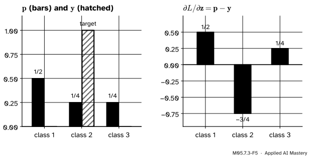
Scores \(\vect{z} = (\ln 2, 0, 0)\) give \(\vect{p} = (1/2, 1/4, 1/4)\). With target class 2 the gradient is \(\vect{p} - \vect{y} = (1/2, -3/4, 1/4)\): gradient descent raises the score of the true class and lowers the others, each in proportion to its probability.
An elementwise activation. If \(\mat{A} = \sigma(\mat{Z})\) entry by entry, then \({dA_{ij}} = {\sigma'(Z_{ij})\, dZ_{ij}}\), written \(d\mat{A} = \sigma'(\mat{Z}) \circ d\mat{Z}\) with \(\circ\) the entrywise product. Given \(\mat{G}_A = \partial L / \partial \mat{A}\), the change is \({\sum_{ij} (G_A)_{ij}\, \sigma'(Z_{ij})\, dZ_{ij}}\), so
\[
\nabla_{\mat{Z}} L = \mat{G}_A \circ \sigma'(\mat{Z}) .
\]
Layer, activation, softmax with cross-entropy: these three rules are all that M05.9.2 needs to backpropagate through a whole network.
Worked example
A batch of two examples with three inputs and two outputs:
and \(\vect{b} = (\ln 3, 0)\), about \((1.10, 0)\). Example 1 belongs to class 1, example 2 to class 2.
M05.7.3-F3
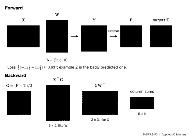
The whole trace. Forward: scores, probabilities, loss. Backward: \(\mat{G}\), then the three products of the theorem, each with the shape of the thing it belongs to.
Forward. Both rows of \(\mat{X}\mat{W}\) are \((1, 1)\): for row 1, \({1 \cdot 1 + 0 \cdot 1 + 2 \cdot 0} = 1\) and \({1 \cdot (-1) + 0 + 2 \cdot 1} = 1\); row 2 is similar. Adding \(\vect{b}\) gives the scores \((1 + \ln 3,\; 1)\) for both examples. Softmax divides by the total: \(e^{1 + \ln 3} = 3e\), so \(\vect{p} = (3e, e)/(4e) = (3/4, 1/4)\) for each example. The loss is the mean of \(-\ln(3/4) \approx 0.288\) and \(-\ln(1/4) \approx 1.386\), about \(0.837\).
Backward.\(\mat{P} - \mat{T}\) has rows \((-1/4, 1/4)\) and \((3/4, -3/4)\); dividing by \(B = 2\),
The third row is \({2 \cdot (-1/8) + 1 \cdot 3/8} = 1/8\) and \({2 \cdot 1/8 + 1 \cdot (-3/8)} = -1/8\). For the input gradient, \(\mat{W}\T\) has rows \((1, 1, 0)\) and \((-1, 0, 1)\), so
For instance the first entry is \({-1/8 \cdot 1 + 1/8 \cdot (-1)} = -1/4\). Finally \(\nabla_{\vect{b}} L = (-1/8 + 3/8,\; 1/8 - 3/8) = (1/4, -1/4)\). A gradient step lowers the bias of class 1: the layer was too sure of class 1, and example 2 paid for it.
The softmax example. For \(\vect{p} = (1/2, 1/4, 1/4)\), \(\operatorname{diag}(\vect{p}) - \vect{p}\vect{p}\T\) has diagonal \({1/2 - 1/4} = 1/4\), \({1/4 - 1/16} = 3/16\) and \(3/16\), and off-diagonal entries \(-1/8\), \(-1/8\) and \(-1/16\). The loss for class 2 is \(-\ln p_2\), whose gradient with respect to \(\vect{p}\) is \((0, -4, 0)\). The chain rule multiplies by the transposed Jacobian, which here is the Jacobian itself because it is symmetric: \(-4\) times its second column is \({(1/2, -3/4, 1/4)} = {\vect{p} - \vect{y}}\).
Code
From scratch: the forward and backward pass of a layer with softmax and mean cross-entropy, on random numbers, checked entry by entry against central differences.
import numpy as npdef softmax(Z):"""Row by row, shifted by each row's largest score so that exp cannot overflow.""" E = np.exp(Z - Z.max(axis=1, keepdims=True))return E / E.sum(axis=1, keepdims=True)def loss(X, W, b, T): P = softmax(X @ W + b)return-np.mean(np.sum(T * np.log(P), axis=1))def backward(X, W, b, T): P = softmax(X @ W + b) G = (P - T) /len(X)return X.T @ G, G @ W.T, G.sum(axis=0)def num_grad(f, V, h=1e-6): G = np.zeros_like(V)for index in np.ndindex(V.shape): E = np.zeros_like(V) E[index] = h G[index] = (f(V + E) - f(V - E)) / (2* h)return Grng = np.random.default_rng(5)B, d, m =5, 4, 3X, W, b = rng.normal(size=(B, d)), rng.normal(size=(d, m)), rng.normal(size=m)T = np.eye(m)[rng.integers(0, m, size=B)] # one-hot targetsdW, dX, db = backward(X, W, b, T)checks = {"W": (dW, num_grad(lambda V: loss(X, V, b, T), W)),"X": (dX, num_grad(lambda V: loss(V, W, b, T), X)),"b": (db, num_grad(lambda V: loss(X, W, V, T), b)),}for name, (formula, numeric) in checks.items():print(f"gradient for {name}: shape {formula.shape}, largest gap {np.abs(formula - numeric).max():.1e}")
gradient for W: shape (4, 3), largest gap 3.0e-10
gradient for X: shape (5, 4), largest gap 2.5e-10
gradient for b: shape (3,), largest gap 1.7e-11
The worked example, and the softmax Jacobian checked against a numerical Jacobian:
P = [[0.75, 0.25], [0.75, 0.25]]   loss = 0.837
grad W [[-1.0, 1.0], [3.0, -3.0], [1.0, -1.0]] / 8
grad X [[-2.0, -1.0, 1.0], [6.0, 3.0, -3.0]] / 8
grad b [2.0, -2.0] / 8
p = [0.5  0.25 0.25]   16 J = [[4.0, -2.0, -2.0], [-2.0, 3.0, -1.0], [-2.0, -1.0, 3.0]]
largest gap from the numerical Jacobian: 3.5e-11   J^T(-y/p) = [ 0.5  -0.75  0.25]
The same check with SciPy. scipy.special.softmax normalises over the whole array unless told an axis, and scipy.optimize.check_grad returns the length of the difference between a gradient function and a finite-difference one; it wants flat vectors, so the weights are flattened.
from scipy.special import softmax as sp_softmaxfrom scipy.optimize import check_gradZ = X @ W + bprint("axis=1 matches ours:", np.allclose(sp_softmax(Z, axis=1), softmax(Z))," default axis sums to", round(sp_softmax(Z).sum(), 6))err = check_grad(lambda v: loss(X, v.reshape(d, m), b, T),lambda v: backward(X, v.reshape(d, m), b, T)[0].ravel(), W.ravel())print("check_grad on W:", f"{err:.1e}")A_in = rng.normal(size=(B, d))Zh = A_in @ WGa = rng.normal(size=(B, m)) # any upstream gradient for tanh(Z)grad_Z = Ga * (1- np.tanh(Zh) **2)numeric_Z = num_grad(lambda V: np.sum(Ga * np.tanh(V)), Zh)print("tanh: largest gap", f"{np.abs(grad_Z - numeric_Z).max():.1e}")
axis=1 matches ours: True   default axis sums to 1.0
check_grad on W: 6.3e-08
tanh: largest gap 1.7e-10
check_grad uses forward differences with a step of about \({1.5 \times 10^{-8}}\), so its error is larger than that of our central differences, but still tiny.
Explore
The gradient heatmap of M05.7.2 draws gradients with respect to a matrix entry by entry. Its preset \({\norm{\mat{A}\mat{X} - \mat{B}}_F^2}\) is a dense layer with a squared-error loss: its gradient \({2\mat{A}\T(\mat{A}\mat{X} - \mat{B})}\) has the same pattern as \(\mat{X}\T\mat{G}\) here.
Pitfalls
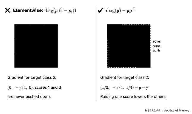
M05.7.3-F4
Wrong beside right. Softmax is not an elementwise function: each probability depends on every score, so its Jacobian has off-diagonal entries, and dropping them changes the gradient.
“Softmax acts entry by entry, so its derivative is \(p_i(1 - p_i)\).”
That is only the diagonal of the Jacobian. Raising one score lowers every other probability, which the off-diagonal entries \(-p_i p_j\) record. With the diagonal alone the gradient in the figure would never push the wrong classes down.
“Softmax over a batch: just call softmax.”
Some library functions normalise over the whole array by default. scipy.special.softmax does: without axis=1, the probabilities of all examples together add to 1, as the code above shows. Normalise each row, one example at a time.
“The bias gradient is the sum of \(\mat{G}\) along any axis.”
Along the batch axis, giving one entry per output: the column sums. Summing along the other axis gives one number per example, \(B\) of them, which cannot be the gradient of a bias with \(m\) entries. Checking the shape catches it.
Check yourself
Recall
1. For \(\mat{Y} = \mat{X}\mat{W} + \vect{1}\vect{b}\T\) and \(\mat{G} = \partial L/\partial\mat{Y}\), what is \(\nabla_{\mat{W}} L\)?
Show answer
\(\mat{X}\T\mat{G}\), with the shape of \(\mat{W}\).
2. What is \(\nabla_{\mat{X}} L\) for the same layer?
Show answer
\(\mat{G}\mat{W}\T\), with the shape of \(\mat{X}\).
4. What is the gradient of cross-entropy after softmax with respect to the scores?
Show answer
\(\vect{p} - \vect{y}\), and \((\mat{P} - \mat{T})/B\) for the mean over a batch.
5. How does a gradient pass back through an elementwise activation \(\sigma\)?
Show answer
As an entrywise product: \(\nabla_{\mat{Z}} L = \mat{G}_A \circ \sigma'(\mat{Z})\).
Exercises
1.★ A layer takes a batch of 32 examples with 10 features to 5 outputs. Give the shapes of \(\mat{X}\), \(\mat{W}\), \(\vect{b}\), \(\mat{G}\) and the three gradients.
2.★★ For two classes, softmax of \((z_1, z_2)\) gives \(p_1 = \sigma(z_1 - z_2)\), the logistic function. Use the softmax Jacobian to show that \(\pd{p_1}{z_1} = \sigma'(z_1 - z_2)\), and find \(\pd{L}{z_1}\) for cross-entropy when the target is class 1.
Show solution
\(p_1 = e^{z_1}/(e^{z_1} + e^{z_2}) = 1/(1 + e^{-(z_1 - z_2)})\). The Jacobian entry is \(\pd{p_1}{z_1} = p_1 - p_1^2 = p_1(1 - p_1)\), which is \(\sigma'(u) = \sigma(u)(1 - \sigma(u))\) at \(u = z_1 - z_2\) (M04.3.3). With \(\vect{y} = (1, 0)\), \(\pd{L}{z_1} = p_1 - 1\).
3.★★★ A loss is the mean squared error of the layer, \(L = \frac{1}{B}\norm{\mat{Y} - \mat{T}}_F^2\). Find \(\mat{G}\) and then \(\nabla_{\mat{W}} L\). For one output (\(m = 1\)) and \(\vect{b} = 0\), compare with the least-squares gradient of M05.7.2.
Show solution
With \(\mat{R} = \mat{Y} - \mat{T}\), \(dL = \frac{2}{B}\operatorname{tr}(\mat{R}\T d\mat{Y})\), as in Gradient 3 of M05.7.2. So \(\mat{G} = \frac{2}{B}(\mat{Y} - \mat{T})\) and \(\nabla_{\mat{W}} L = \frac{2}{B}\mat{X}\T(\mat{Y} - \mat{T})\). For one output, \(\mat{W}\) is a column \(\vect{w}\), \(\mat{Y} = \mat{X}\vect{w}\) and \(\mat{T} = \vect{y}\), so the gradient is \({\frac{2}{B}\mat{X}\T(\mat{X}\vect{w} - \vect{y})}\): least squares, with \(B\) in the role of \(n\).
Summary card
Every gradient is one product, fixed by its shape.
Softmax:\(\mat{J} = \operatorname{diag}(\vect{p}) - \vect{p}\vect{p}\T\); rows sum to 0.
With cross-entropy:\(\partial L/\partial\vect{z} = \vect{p} - \vect{y}\); batch mean \((\mat{P} - \mat{T})/B\).
Activation:\(\nabla_{\mat{Z}} L = \mat{G}_A \circ \sigma'(\mat{Z})\).
Sources and next steps
Sources. Each was opened and checked against this lesson on 15 November 2026.
Christopher M. Bishop, Pattern Recognition and Machine Learning, free PDF from Microsoft Research, Section 4.3.4: the softmax (4.104), its derivatives \(y_k(I_{kj} - y_j)\) in (4.106), the cross-entropy (4.108) and its gradient \({\sum_n (y_{nj} - t_{nj})\,\phi_n}\) in (4.109).
Paige Bright, Alan Edelman and Steven G. Johnson, Matrix Calculus (for Machine Learning and Beyond): Theorem 2 in Section 1.3 (the product rule) and Definition 34 in Section 5.1 (gradients through the Frobenius inner product).
Kaare Brandt Petersen and Michael Syskind Pedersen, The Matrix Cookbook, version of 15 November 2012, Section 2: the differential rules (33) to (38), including (38) for the entrywise product.