Integrate over a triangle, a quarter disc or a tetrahedron by reading the limits off a picture: the inner limits follow the edge of the region. Swap the order by redrawing the slices, compute probabilities of regions under a joint density, and check everything with dblquad and tplquad.
M05.6.2L2 Intermediate25 minIn review (what this means)
The maths and code on this page are checked by automated tests on every change, but an independent reader has not signed it off yet. Spot a mistake or a confusing step? Tell us.
Describe a region bounded by curves as lying between two functions of x or between two functions of y, and read the limits of an iterated integral off its picture.
Reverse the order of integration by redrawing the slices, and choose the order in which the inner integral has a formula.
Compute the probability that a pair of random variables lands in a region, such as X + Y < 1 or X < Y, as a double integral of their joint density.
Set up a triple integral over a box and over a tetrahedron, and evaluate double and triple integrals with function limits in scipy.integrate.dblquad and tplquad.
The question
Two features \(X\) and \(Y\) have a joint density on the unit square. What is the chance that \({X + Y < 1}\), or that \({X < Y}\)? Each is a double integral, but over a triangle, not a rectangle, so the limits of the inner integral can no longer be constants. How do we find them, and does the order of integration still not matter?
From the last lesson
1. What does Fubini’s theorem say for a continuous \(f\) on a rectangle?
Show answer
The double integral equals either iterated integral: \(y\) inside and \(x\) outside, or the reverse.
2. How does scipy.integrate.dblquad expect its integrand?
Show answer
As func(y, x), with the inner variable \(y\) first.
Intuition
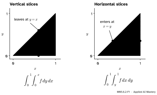
Slicing still works on any region. Fix \(x\) and draw the vertical line at that \(x\): it enters the region at one edge and leaves at another, and those two edges are the limits of the inner integral. They depend on \(x\) now, because the region is not a rectangle.
M05.6.2-F1
One triangle, \({0 < y < x < 1}\), sliced two ways. Vertical slices run from \({y = 0}\) up to \({y = x}\); horizontal slices run from \({x = y}\) across to \({x = 1}\). The limits come from the picture, not from the formula for \(f\).
Slice the other way, horizontally, and the edges where a slice enters and leaves change. So swapping the order of integration means redrawing the slices, not swapping the symbols.
Build it up
Step 1. Put the region in a rectangle. Let \(D\) be a region inside a rectangle \(R\). Define a new function equal to \(f\) on \(D\) and to 0 outside it. Its integral over \(R\) is, by definition, the integral of \(f\) over \(D\). In a Riemann sum, cells inside \(D\) count, cells outside add nothing, and only cells that straddle the edge cause trouble. For a region bounded by smooth curves their total area shrinks to 0 as the cells shrink, so they do not matter in the limit.
Step 2. Draw the region and one slice. Draw \(D\). Draw the vertical line at a typical \(x\). Mark where it enters \(D\) (the lower edge, \({y = g_1(x)}\)) and where it leaves (the upper edge, \({y = g_2(x)}\)).
Step 3. Read the outer limits. Slide the line from the leftmost \(x\) that meets \(D\) to the rightmost. Those two numbers, \(a\) and \(b\), are the outer limits. They are constants: the outer integral must give a number.
M05.6.2-F2
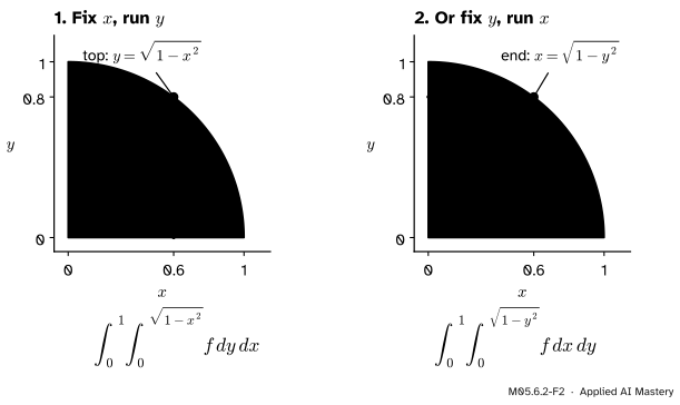
Reading the limits for the quarter disc. The circle \({x^2 + y^2 = 1}\) gives the top of a vertical slice, \({y = \sqrt{1 - x^2}}\), and the end of a horizontal slice, \({x = \sqrt{1 - y^2}}\).
Step 4. To swap the order, redraw. Draw a horizontal line at a typical \(y\) instead, and read the left edge \({x = h_1(y)}\) and the right edge \({x = h_2(y)}\) where it enters and leaves. The outer limits are now the lowest and highest \(y\) in \(D\).
The formal statement
NoteDefinition: regions between two curves
A region is of type I when it lies between two vertical lines and two continuous curves: \({a \le x \le b}\) and \({g_1(x) \le y \le g_2(x)}\). It is of type II when it lies between two horizontal lines and two continuous curves: \({c \le y \le d}\) and \({h_1(y) \le x \le h_2(y)}\).
NoteTheorem: Fubini, for regions between curves
If \(f\) is continuous on a type I region \(D\), then
Why. Step 1 turned the integral over \(D\) into an integral over a rectangle of a function that is 0 outside \(D\). Apply Fubini for rectangles with \(y\) inside: for fixed \(x\), the inner integrand is 0 except between \({g_1(x)}\) and \({g_2(x)}\), so the inner integral only runs between them. (The new function jumps at the edge of \(D\), but only along a curve, whose cells add nothing in the limit by Step 1. OpenStax states the result as the strong form of Fubini’s theorem.)
A region that is of both types, like the triangle and the quarter disc, can be integrated in either order with the same answer. With \({f = 1}\) the inner integral is the length of the slice, so the area of \(D\) is \({\int_a^b \big(g_2(x) - g_1(x)\big)\,dx}\): the area between two curves.
Probabilities of regions. If \(X\) and \(Y\) have joint density \(p\) (M06.9.4), then for any region \(D\)
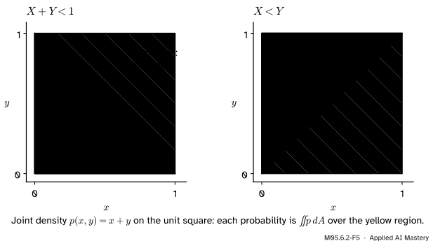
Take \({p(x, y) = x + y}\) on the unit square, a density because its integral over the square is \({\tfrac12 + \tfrac12 = 1}\). For \({X + Y < 1}\), a vertical slice runs from \({y = 0}\) to \({y = 1 - x}\), and the inner integral is
as the symmetry of \(p\) in \(x\) and \(y\) says it must be.
M05.6.2-F5
Two events as two regions. The triangle \({X + Y < 1}\) has half the area of the square but only a third of the probability, because it sits where the density is low.
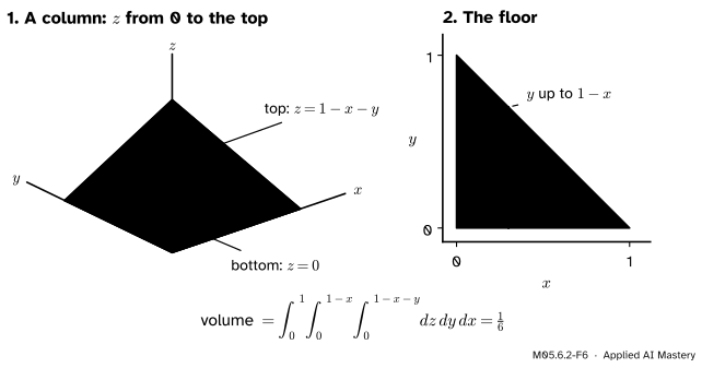
Triple integrals. One more variable adds one more layer. Over a box, Fubini gives three nested integrals in any order, for example \({\iiint xyz\,dV = \big(\tfrac12\big)^3 = \tfrac18}\) over the unit cube. Over the tetrahedron \({x, y, z \ge 0}\), \({x + y + z \le 1}\), a vertical column at \({(x, y)}\) runs from \({z = 0}\) to \({z = 1 - x - y}\), and the floor is the triangle under \({y = 1 - x}\):
Here \(V\) is the volume, and the inner integral is over \(y\) after the innermost one over \(z\) has given the column’s height \({1 - x - y}\).
M05.6.2-F6
A triple integral is read the same way, one layer at a time: the column gives the limits for \(z\), and the floor below it is an ordinary region of the plane.
Worked example
\({\iint xy\,dA}\) over the triangle \({0 < y < x < 1}\), both orders. With vertical slices, \(y\) runs from 0 to \(x\):
So the average of \(x\) over the quarter disc is \({\tfrac13 \big/ \tfrac{\pi}{4} = \tfrac{4}{3\pi} \approx 0.424}\): the balance point of the region sits a little left of the middle.
An integral that goes only one way. Integrate \({e^{-x^2}}\) over the same triangle. With \(y\) inside, the integrand does not depend on \(y\), so the inner integral is the slice length times the height: \({\int_0^x e^{-x^2}\,dy = x\,e^{-x^2}}\), and then
With \(x\) inside, the first step would be \({\int_y^1 e^{-x^2}\,dx}\), which has no formula in elementary functions (M04.7.4). Same region, same answer, but only one order can be done by hand.
M05.6.2-F3
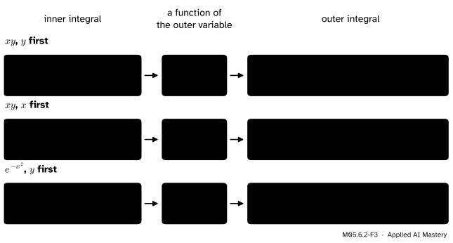
The worked examples as a trace. Both orders give \({\tfrac18}\) for \(xy\); for \({e^{-x^2}}\) only the order with \(y\) inside reaches a formula.
Code
dblquad takes function limits for the inner variable: gfun(x) and hfun(x) are the lower and upper edges of a slice. For the other order, rename the roles: the outer variable is whatever the second argument of the integrand is.
import mathfrom scipy.integrate import dblquad, tplquad# x y over the triangle 0 < y < x < 1y_first = dblquad(lambda y, x: x * y, 0, 1, 0, lambda x: x)[0] # x outside, y from 0 to xx_first = dblquad(lambda x, y: x * y, 0, 1, lambda y: y, 1)[0] # y outside, x from y to 1quarter_area = dblquad(lambda y, x: 1.0, 0, 1, 0, lambda x: math.sqrt(1- x**2))[0]quarter_x = dblquad(lambda y, x: x, 0, 1, 0, lambda x: math.sqrt(1- x**2))[0]bell_tri = dblquad(lambda y, x: math.exp(-x**2), 0, 1, 0, lambda x: x)[0]p =lambda y, x: x + y # the joint density, y firstbelow = dblquad(p, 0, 1, 0, lambda x: 1- x)[0] # X + Y < 1above = dblquad(p, 0, 1, lambda x: x, 1)[0] # X < Yprint(round(y_first, 10), round(x_first, 10), round(quarter_area, 6), round(quarter_x / quarter_area, 4))print(round(bell_tri, 4), round(below, 10), round(above, 10))
tplquad(func, a, b, gfun, hfun, qfun, rfun) adds a layer: func(z, y, x) takes the innermost variable first, \(y\) runs from gfun(x) to hfun(x), and \(z\) from qfun(x, y) to rfun(x, y). Note the order of those last arguments: \(x\) first.
cube = tplquad(lambda z, y, x: x * y * z, 0, 1, 0, 1, 0, 1)[0]tet = tplquad(lambda z, y, x: 1.0, 0, 1, 0, lambda x: 1- x, 0, lambda x, y: 1- x - y)[0]tet_x = tplquad(lambda z, y, x: x, 0, 1, 0, lambda x: 1- x, 0, lambda x, y: 1- x - y)[0]print(round(cube, 10), round(tet, 10), round(tet_x, 10), " mean of x:", round(tet_x / tet, 10))
0.125 0.1666666667 0.0416666667 mean of x: 0.25
Explore
The region integrator in lesson M05.6.3 covers the triangle of this lesson with Cartesian cells. Watch the cells cut by the diagonal: each counts in full or not at all. On an \({n \times n}\) grid the \(n\) cells along the diagonal all count, so the sum for \({f = 1}\) is \({\tfrac12 + \tfrac{1}{2n}}\): too big by half of those cells, an error that shrinks only like \({1/n}\).
Pitfalls
M05.6.2-F4
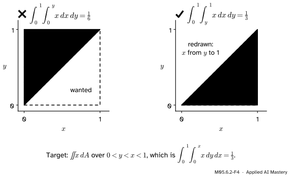
Wrong beside right. Swapping \({dy\,dx}\) for \({dx\,dy}\) and renaming the limits integrates over the other triangle and gives \({\tfrac16}\); redrawing the slices gives the right \({\tfrac13}\).
“To swap the order, swap \(dx\) and \(dy\) and the letters in the limits.”
The limits describe the region, so they must be read again from a picture. From \({\int_0^1 \int_0^x f\,dy\,dx}\), renaming gives \({\int_0^1 \int_0^y f\,dx\,dy}\), which covers \({0 < x < y < 1}\), the wrong triangle. Redrawn, the triangle’s horizontal slices run from \({x = y}\) to \({x = 1}\).
“The outer limits can depend on the inner variable.”
Never. After the inner integral the inner variable is gone, so an outer limit that mentions it is meaningless. Only the inner limits may depend on the outer variable; the outermost limits are always numbers.
“tplquad passes its arguments in the same order everywhere.”
The integrand takes (z, y, x), innermost first, but the \(z\) limits qfun and rfun take (x, y), outermost first. Writing lambda y, x: 1 - x - y happens to work for the symmetric tetrahedron and fails silently for a region like \({z \le 1 - 2x - y}\).
Check yourself
Recall
1. For a vertical slice at a fixed \(x\), where do the limits of the inner integral come from?
Show answer
From where the vertical line enters and leaves the region: the lower edge \({y = g_1(x)}\) and the upper edge \({y = g_2(x)}\).
2. Write the triangle \({0 < y < x < 1}\) as a type II region.
Show answer
\({0 \le y \le 1}\) and \({y \le x \le 1}\).
3. What is \({\iint xy\,dA}\) over that triangle?
Show answer
\({\tfrac18}\), in either order.
4. How is the probability that \({(X, Y)}\) lands in a region \(D\) computed from a joint density \(p\)?
Show answer
As \({\iint_D p\,dA}\). For \({p = x + y}\) on the unit square, \({\Prob(X + Y < 1) = \tfrac13}\).
5. Why can \({\iint e^{-x^2}\,dA}\) over the triangle under \({y = x}\) be done only with \(y\) inside?
Show answer
With \(y\) inside the inner integral is \({x\,e^{-x^2}}\), which has an antiderivative; with \(x\) inside the first step is \({\int e^{-x^2}\,dx}\), which has no elementary formula.
Exercises
1.★ Find the area between \({y = x^2}\) and \({y = x}\) for \({0 \le x \le 1}\) as a double integral.
Show solution
For \({0 < x < 1}\) the line is above the parabola, so a vertical slice runs from \({y = x^2}\) to \({y = x}\). The area is \({\int_0^1 \int_{x^2}^{x} 1\,dy\,dx} = {\int_0^1 (x - x^2)\,dx} = {\tfrac12 - \tfrac13} = \tfrac16\).
2.★★ Evaluate \({\int_0^1 \int_x^1 \sin(y^2)\,dy\,dx}\) by reversing the order.
Show solution
The inner integral has no elementary formula, so redraw. The region is \({0 \le x \le 1}\), \({x \le y \le 1}\): the triangle above the diagonal. A horizontal slice at height \(y\) runs from \({x = 0}\) to \({x = y}\). So the integral is \({\int_0^1 \int_0^y \sin(y^2)\,dx\,dy} = {\int_0^1 y\sin(y^2)\,dy}\). With \({u = y^2}\) this is \({\tfrac12\int_0^1 \sin u\,du} = {\tfrac{1 - \cos 1}{2}} \approx 0.2298\).
3.★★★ A point is chosen uniformly in the tetrahedron \({x, y, z \ge 0}\), \({x + y + z \le 1}\), so its density is 6 there. Find \({\E[X]}\).
Show solution
\({\E[X] = \iiint 6x\,dV}\). The inner integral in \(z\) is \({x(1 - x - y)}\). Then
Sources. Each was opened and checked against this lesson on 15 November 2026.
Gilbert Strang and Edwin Herman, Calculus Volume 3, Section 5.2, Double integrals over general regions, OpenStax. Type I and type II regions, and Fubini’s theorem in its strong form for them (Theorem 5.4); Example 5.15 reverses the order to make an integral easy. Section 5.4, Triple integrals: Fubini’s theorem for a box (Theorem 5.9) and a triple integral over the tetrahedron bounded by the coordinate planes and \({x + y + z = 1}\) (Example 5.38).
SciPy reference, scipy.integrate.dblquad (function limits gfun(x), hfun(x) for \(y\)) and scipy.integrate.tplquad: func(z, y, x), with the \(z\) limits qfun and rfun taking \({(x, y)}\).