The volume under a surface over a rectangle is the limit of sums of thin boxes, and Fubini’s theorem computes it one slice at a time, in either order. Worked on x y and the running bowl over the unit square, checked with midpoint sums and scipy.integrate.dblquad.
M05.6.1L2 Intermediate25 minIn review (what this means)
The maths and code on this page are checked by automated tests on every change, but an independent reader has not signed it off yet. Spot a mistake or a confusing step? Tell us.
Define the double integral over a rectangle as the limit of double Riemann sums, and compute a midpoint sum on a grid by hand and with NumPy.
State Fubini’s theorem for a continuous function on a rectangle and evaluate a double integral as an iterated integral in either order.
Find the average value of a function over a rectangle, and read an expectation under a joint density as a double integral.
Call scipy.integrate.dblquad correctly, knowing that its integrand takes the inner variable y first.
The question
The running bowl \({f(x, y) = x^2 + 2y^2}\) rises from 0 at one corner of the unit square to 3 at the opposite one. How much space is there under it, above the square? And what is its average height there? The same question, asked of a density, is how machine learning computes an expectation of two random inputs, such as the mean loss over a joint distribution of features.
Intuition
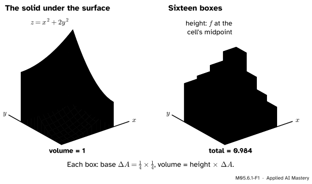
In one variable, the area under a curve was a limit of thin rectangles (M04.5.2). In two variables, the graph of \(f\) is a surface above the plane, and the question is a volume. The same trick works: cut the square into a grid of cells, stand a box on each cell as tall as the surface above it, and add up the volumes of the boxes.
M05.6.1-F1
The solid under the running bowl (left) and sixteen boxes that imitate it (right). Each box takes its height from the surface above the midpoint of its cell. The boxes hold 0.984; the solid holds exactly 1.
The boxes are too small where the surface curves up between midpoints and too big where it dips, and the two nearly cancel. Make the cells smaller and the staircase of boxes hugs the surface more closely. The volume it approaches is the double integral.
Build it up
Step 1. Cut the rectangle into cells. Take a rectangle \({[a, b] \times [c, d]}\) (all points with \({a \le x \le b}\) and \({c \le y \le d}\)). Cut \({[a, b]}\) into \(m\) equal pieces of width \({\Delta x = (b - a)/m}\) and \({[c, d]}\) into \(n\) pieces of height \({\Delta y = (d - c)/n}\). The rectangle becomes \({mn}\) cells, each of area \({\Delta A = \Delta x\,\Delta y}\).
Step 2. Give each cell a height. Pick a sample point \({(x_{ij}^*, y_{ij}^*)}\) in cell \({(i, j)}\). The box on that cell has volume \({f(x_{ij}^*, y_{ij}^*)\,\Delta A}\). Taking the midpoint of each cell gives the midpoint sum, as in one variable.
Step 3. Add the boxes. The total is a double Riemann sum:
\[
\sum_{i=1}^{m} \sum_{j=1}^{n} f(x_{ij}^*, y_{ij}^*)\,\Delta A .
\]
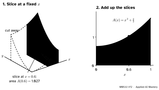
Step 4. Group the boxes by column. Fix one value of \(i\), a column of cells at the same \(x\). Its \(n\) boxes add up to \({\big(\sum_j f(x_i^*, y_j^*)\,\Delta y\big)\,\Delta x}\), and the bracket is a one-variable Riemann sum in \(y\). As the cells shrink it becomes the area of the slice of the solid at that \(x\). Adding the columns then becomes adding up slice areas across \(x\).
M05.6.1-F2
Fubini’s idea in two steps. The slice at a fixed \(x\) has area \({A(x) = x^2 + \tfrac{2}{3}}\), an ordinary integral in \(y\). The volume is the area under the curve \(A(x)\), an ordinary integral in \(x\).
So a double integral is two single integrals, one inside the other. Each is the kind of integral the fundamental theorem of calculus (M04.6) already handles.
The formal statement
NoteDefinition: double integral over a rectangle
Let \(f\) be defined on \({D = [a, b] \times [c, d]}\). If the double Riemann sums approach one number as \({m}\) and \(n\) grow, whatever sample points are chosen, that number is the double integral
\[
\begin{aligned}
&\iint_D f(x, y)\,dA \\
&\quad= \lim_{m, n \to \infty} \sum_{i=1}^{m} \sum_{j=1}^{n} f(x_{ij}^*, y_{ij}^*)\,\Delta A .
\end{aligned}
\]
Every continuous \(f\) has one. Where \({f \ge 0}\) it is the volume under the graph and above \(D\).
NoteTheorem: Fubini, for rectangles
If \(f\) is continuous on \({D = [a, b] \times [c, d]}\), then
The right-hand sides are iterated integrals. In the inner integral the outer variable is held fixed, exactly as a partial derivative holds the other input fixed (M04.10.2), so the result is a function of the outer variable alone. The brackets are usually dropped: \({\int_a^b \int_c^d
f\,dy\,dx}\) means \(y\) inside, \(x\) outside.
Why it holds. Step 4 of the build grouped the double sum by columns,
\[
\sum_{i=1}^{m} \Big( \sum_{j=1}^{n} f(x_i^*, y_j^*)\,\Delta y \Big)\,\Delta x .
\]
For continuous \(f\), the bracket tends to \({A(x_i^*) = \int_c^d f(x_i^*, y)\,dy}\) as \(n\) grows, at the same rate for every column. What is left is a Riemann sum of \(A\), which tends to \({\int_a^b A(x)\,dx}\). Grouping by rows instead gives the other order.
Go deeper: what 'at the same rate for every column' needs
A continuous function on a closed rectangle is uniformly continuous: for every tolerance \({\varepsilon > 0}\) there is a cell size below which \(f\) changes by less than \(\varepsilon\) inside any cell, wherever the cell is. Then each box differs from the true volume over its cell by less than \({\varepsilon\,\Delta A}\), so the whole sum is within \({\varepsilon\,(b - a)(d - c)}\) of the volume, for any grouping of the boxes. Courses in real analysis turn this into a full proof. Without continuity the two orders can disagree, as the second pitfall shows.
Two consequences. If \({f(x, y) = g(x)\,h(y)}\), the inner integral pulls \(g(x)\) out as a constant, so the integral factorises:
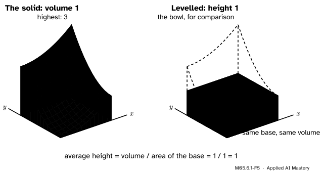
Levelling the solid. The bowl runs from 0 to 3 over the unit square, but a box of height 1 on the same base holds the same volume, so its average height is 1.
For a joint density \(p\) of two inputs on \(D\) (M06.9.4), the same integral with a weight gives an expectation: \({\E[g(X, Y)] = \iint_D g\,p\,dA}\). Under the uniform density \({p = 1}\) on the unit square, an average over the square is an expectation.
Worked example
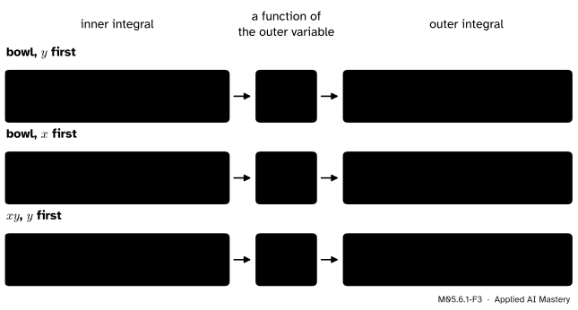
The running bowl over the unit square, in both orders. With \(y\) inside, \(x\) is a constant and \({\int_0^1 2y^2\,dy = \tfrac{2}{3}}\):
Each inner integral leaves a function of the outer variable alone (middle column); the outer integral turns it into a number. Both orders give 1 for the bowl.
Read as expectations. If \(X\) and \(Y\) are independent and uniform on \({[0, 1]}\), their joint density is 1 on the square (M06.9.4). Then \({\E[XY] = \tfrac14}\), which is \({\E[X]\,\E[Y]}\), and \({\E[X^2 + 2Y^2] = 1}\).
The boxes of the anchor picture. With \({4 \times 4}\) cells, the midpoints are \(\tfrac18\), \(\tfrac38\), \(\tfrac58\) and \(\tfrac78\) in each direction. Exercise 3 shows that \(n \times n\) midpoint cells give exactly \({1 - \tfrac{1}{4n^2}}\) for the bowl, so \({1 - \tfrac{1}{64} = 0.984375}\) here. The error \({\tfrac{1}{4n^2}}\) falls by a factor of 4 each time \(n\) doubles.
Code
From scratch: the midpoint sum on an \({n \times n}\) grid, built with numpy.meshgrid.
import numpy as npdef midpoint_sum(f, a, b, c, d, n):"""Midpoint double Riemann sum of f over [a, b] x [c, d] with n x n cells.""" dx, dy = (b - a) / n, (d - c) / n xs = a + dx * (np.arange(n) +0.5) # the midpoints in x ys = c + dy * (np.arange(n) +0.5) # the midpoints in y X, Y = np.meshgrid(xs, ys) # every cell's midpointreturn np.sum(f(X, Y)) * dx * dybowl =lambda x, y: x**2+2* y**2print(" n sum error n^2 * error")for n in [1, 2, 4, 8, 16, 32]: s = midpoint_sum(bowl, 0, 1, 0, 1, n)print(f"{n:2d}{s:.6f}{1- s:.6f}{n**2* (1- s):.4f}")print("x y with 3 x 3 cells:", midpoint_sum(lambda x, y: x * y, 0, 1, 0, 1, 3))
 n   sum        error      n^2 * error
 1  0.750000   0.250000   0.2500
 2  0.937500   0.062500   0.2500
 4  0.984375   0.015625   0.2500
 8  0.996094   0.003906   0.2500
16  0.999023   0.000977   0.2500
32  0.999756   0.000244   0.2500
x y with 3 x 3 cells: 0.24999999999999992
The last column stays at 0.25: the error is \({\tfrac{1}{4n^2}}\), the observed rate of order \(n^{-2}\). For \(xy\) the midpoint sum is exact for every grid, because the midpoint rule is exact for a function that is linear in each variable.
The library: scipy.integrate.dblquad(func, a, b, gfun, hfun) integrates over \({a \le x \le b}\) and \({\text{gfun}(x) \le y \le \text{hfun}(x)}\), with func(y, x): the inner variable comes first.
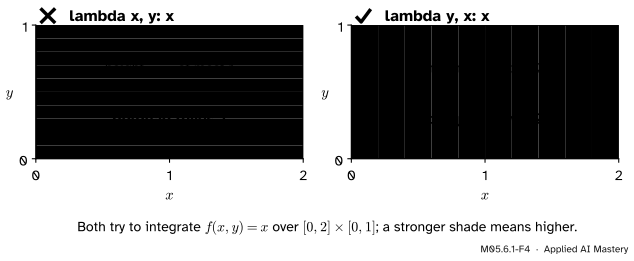
from scipy.integrate import dblquadvalue, err = dblquad(lambda y, x: x**2+2* y**2, 0, 1, 0, 1)print("bowl:", round(value, 12), " x y:", round(dblquad(lambda y, x: x * y, 0, 1, 0, 1)[0], 12))# f(x, y) = x over [0, 2] x [0, 1]: the order of the lambda's arguments matterswrong = dblquad(lambda x, y: x, 0, 2, 0, 1)[0]right = dblquad(lambda y, x: x, 0, 2, 0, 1)[0]print("lambda x, y:", round(wrong, 12), " lambda y, x:", round(right, 12))
bowl: 1.0  x y: 0.25
lambda x, y: 1.0   lambda y, x: 2.0
Finally, a function for which the two orders disagree (the second pitfall). The inner integrals are done by antiderivative: the derivative of \({y/(x^2 + y^2)}\) with respect to \(y\) is \({(x^2 - y^2)/(x^2 + y^2)^2}\) (quotient rule), so the inner integral in \(y\) is \({1/(x^2 + 1)}\). With the roles swapped the integrand changes sign, and the inner integral in \(x\) is \({-1/(1 + y^2)}\).
This module’s interactive, the region integrator, lives in lesson M05.6.3. On the rectangle with Cartesian cells it is this lesson’s picture seen from above: slide the number of cells and watch the midpoint sum of the bowl close in on 1, its error falling about fourfold each time the cells double.
Pitfalls
M05.6.1-F4
Wrong beside right. dblquad fills the first argument with \(y\). Written as lambda x, y: x, the function returns \(y\) and the answer is 1 instead of 2.
“dblquad takes f(x, y), like everything else.”
It takes func(y, x): the variable of the inner integral first. A function written f(x, y) is evaluated with the two inputs swapped, which changes the answer unless \(f\) happens to be symmetric and the region square. Write the lambda as lambda y, x: ... every time, or wrap your function: lambda y, x: f(x, y).
“The order of integration never matters.”
Fubini’s theorem needs a condition: continuity on the closed rectangle (or, more generally, a finite integral of \({\abs{f}}\)). The function \({(x^2 - y^2)/(x^2 + y^2)^2}\) on the unit square blows up at the origin. With \(y\) inside, its iterated integral is \({\pi/4}\); with \(x\) inside it is \({-\pi/4}\) (the last code cell). Neither is the double integral, because there is none.
“A double integral is an area.”
It is a volume, and only \({\iint_D 1\,dA}\) is the area of \(D\). Where \(f\) is negative the boxes count negatively, so the double integral is a signed volume: \({\iint (x - \tfrac12)\,dA = 0}\) over the unit square, though the solid between the plane and the surface is not empty.
Check yourself
Recall
1. What is the volume of one box in a double Riemann sum?
Show answer
The height of \(f\) at the cell’s sample point times the cell’s area: \({f(x_{ij}^*, y_{ij}^*)\,\Delta A}\), with \({\Delta A = \Delta x\,\Delta y}\).
2. What does Fubini’s theorem say for a continuous \(f\) on a rectangle?
Show answer
The double integral equals either iterated integral: \(y\) inside and \(x\) outside, or the reverse.
3. In \({\int_0^1 \int_0^2 f\,dy\,dx}\), which variable runs from 0 to 2, and which is held fixed in the inner integral?
Show answer
\(y\) runs from 0 to 2 in the inner integral, with \(x\) held fixed; then \(x\) runs from 0 to 1.
4. What are the volume and the average height of the running bowl over the unit square?
Show answer
Volume 1. The square has area 1, so the average height is \({1/1 = 1}\).
5. How does scipy.integrate.dblquad expect its integrand?
Show answer
As func(y, x), with the inner variable \(y\) first; \(x\) runs from a to b, \(y\) from gfun(x) to hfun(x).
Exercises
1.★ Compute \({\iint_D (x + 3y)\,dA}\) over \({D = [0, 2] \times [0, 1]}\) and the average value of \({x + 3y}\) on \(D\).
Show solution
With \(y\) inside: \({\int_0^1 (x + 3y)\,dy = x + \tfrac32}\). Then \({\int_0^2 (x + \tfrac32)\,dx} = {2 + 3} = 5\). The area of \(D\) is 2, so the average value is \({5/2 = 2.5}\). (Check: \({x + 3y}\) is linear, so its average is its value at the centre \({(1, \tfrac12)}\), which is \({1 + 1.5 = 2.5}\).)
2.★★ Compute the midpoint sum of the bowl \({x^2 + 2y^2}\) over the unit square with \({2 \times 2}\) cells by hand.
Show solution
The midpoints are \(\tfrac14\) and \(\tfrac34\) in each direction and \({\Delta A = \tfrac14}\). The four heights are \({\tfrac{1}{16} + \tfrac{2}{16} = \tfrac{3}{16}}\), \({\tfrac{9}{16} + \tfrac{2}{16} = \tfrac{11}{16}}\), \({\tfrac{1}{16} + \tfrac{18}{16} = \tfrac{19}{16}}\) and \({\tfrac{9}{16} + \tfrac{18}{16} = \tfrac{27}{16}}\). They add to \({\tfrac{60}{16} = \tfrac{15}{4}}\), and \({\tfrac{15}{4} \times \tfrac14} = \tfrac{15}{16} = 0.9375\), which is \({1 - \tfrac{1}{4 \cdot 2^2}}\).
3.★★★ Prove that the \({n \times n}\) midpoint sum of the bowl over the unit square is exactly \({1 - \tfrac{1}{4n^2}}\). You may use \({\sum_{k=1}^{n} k^2} = {n(n + 1)(2n + 1)/6}\) (M04.5.2).
Show solution
The midpoints are \({(2k - 1)/(2n)}\) for \({k = 1, \dots, n}\). First the odd squares: the squares up to \({2n}\) minus the even squares \({4k^2}\) up to \(n\) give
In the double sum the term \(x_i^2\) does not depend on \(j\), so summing over \(j\) multiplies it by \(n\), and \({n \cdot \Delta A = \tfrac1n}\): the \(x^2\) part is the one-variable sum above. The same holds for \({2y_j^2}\), giving twice that sum. Altogether \({3\big(\tfrac13 - \tfrac{1}{12n^2}\big)} = {1 - \tfrac{1}{4n^2}}\).
Summary card
Volume under a surface: add thin boxes, or add slices.
Average.\({f_{\text{avg}}} = {\iint_D f\,dA \,/\, \text{area}(D)}\); the bowl’s is 1.
SciPy.dblquad(lambda y, x: ..., a, b, c, d): the inner variable first.
Sources and next steps
Sources. Each was opened and checked against this lesson on 15 November 2026.
Gilbert Strang and Edwin Herman, Calculus Volume 3, Section 5.1, Double integrals over rectangular regions, OpenStax. The double integral as the limit of double Riemann sums (equation 5.1), Fubini’s theorem for a continuous function on a rectangle (Theorem 5.2), and the average value over a region (equation 5.4).
SciPy reference, scipy.integrate.dblquad: the signature dblquad(func, a, b, gfun, hfun), with \(y\) the first argument of func and \(x\) the second, constant or function limits for \(y\), and the value returned with an error estimate.