Differentiate the mean squared error of a linear model one weight at a time with the chain rule, then see the whole gradient appear as one matrix product, (2/n) X-transpose r. The mean log loss of logistic regression gives the same shape: (1/n) X-transpose (p - y).
M05.2.3L2 Intermediate25 minIn review (what this means)
The maths and code on this page are checked by automated tests on every change, but an independent reader has not signed it off yet. Spot a mistake or a confusing step? Tell us.
Differentiate the mean squared error of a linear model with d features weight by weight, by the chain rule.
Recognise the n-term sums as the matrix product (2/n) Xᵀr, with the residual vector r = Xw - y and a column of ones for the bias.
Derive the gradient of the mean log loss of logistic regression, (1/n) Xᵀ(p - y), from σ’ = σ(1 - σ).
Evaluate both gradients by hand on small data and check every shape.
Write each gradient as a loop over examples and as one vectorised NumPy expression, and show that they agree.
The question
A linear model with \(d\) features has \({d + 1}\) weights, and its loss averages over \(n\) examples. Each partial derivative is therefore a sum of \(n\) terms, and there are \({d + 1}\) of them. With a thousand features and a million examples, that is a billion terms per step. Is there a way to see the whole gradient at once, as one object that a computer can produce in a single line?
From the last lesson
1. What is the linear model of \(f\) at \(\vect{a}\), and what is its remainder?
Show answer
\({f(\vect{a}) + \nabla f(\vect{a})\T\vect{h}}\); the remainder is \({f(\vect{a} + \vect{h})}\) minus that.
2. What is the tangent plane of the running bowl at \({(1, 1)}\)?
Show answer
\({z = 3 + 2(x - 1) + 4(y - 1)}\), that is \({z = 2x + 4y - 3}\).
Intuition
A weight affects the loss only through the predictions, and it affects each prediction in proportion to the feature it multiplies. So its partial derivative is an average over the examples of two things multiplied: how wrong the prediction is (the residual) and how much of that weight’s feature the example has.
Do this for every weight and stack the answers. Each answer is a column of the data dotted with the residuals, so the stack is one matrix product: the data matrix, transposed, times the residual vector.
M05.2.3-F1
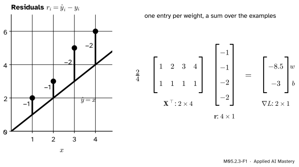
The running loss at \({(w, b) = (1, 0)}\), the line \({\hat y = x}\). Each residual is a prediction minus its target. The gradient is \({\tfrac24\,\mat{X}\T\vect{r}}\): the row of \(x\) values dotted with the residuals gives the entry for \(w\), the row of ones gives the entry for \(b\).
Build it up
Step 1. One example, one weight. The model predicts \({\hat y_i = \vect{w}\T\vect{x}_i + b}\), and example \(i\) contributes \({r_i^2}\) to the loss, with the residual\({r_i = \hat y_i - y_i}\). Only \({\hat y_i}\) depends on \(w_j\), through the term \({w_jx_{ij}}\), so \({\pd{r_i}{w_j} = x_{ij}}\) and \({\pd{r_i}{b} = 1}\). By the chain rule (M04.3.4),
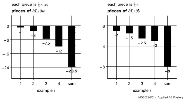
On the running loss at the origin every prediction is 0, so \({r_i = -y_i}\): the residuals are \({(-2, -3, -5, -6)}\). Each example’s piece is \({\tfrac24 r_ix_i}\) for \(w\) and \({\tfrac24 r_i}\) for \(b\).
M05.2.3-F2
Each example’s share of the two partial derivatives at the origin. Examples with large \(x\) and large residuals pull hardest on \(w\). The sums are the gradient \({(-23.5, -8)}\) that M04.10 found.
Step 3. See the matrix. Put the examples in the rows of a matrix: row \(i\) is \({(x_{i1}, \dots, x_{id}, 1)}\), the features followed by a 1. Call it the design matrix\(\mat{X}\), of shape \({n \times (d + 1)}\). Column \(j\) of \(\mat{X}\) holds feature \(j\) for every example, and the sum \({\sum_i x_{ij}r_i}\) in Step 2 is that column dotted with \(\vect{r}\). The dot products of every column of \(\mat{X}\) with \(\vect{r}\), stacked, are exactly \({\mat{X}\T\vect{r}}\). The last column, all ones, gives \({\sum_i r_i}\): the bias needs no separate formula.
The formal statement
NoteResult: the gradient of the mean squared error
Fold the bias into the weights, \({\vect{w} = (w_1, \dots, w_d, b)}\), so that the predictions are \({\mat{X}\vect{w}}\). With the residual vector \({\vect{r} = \mat{X}\vect{w} - \vect{y}}\),
Derivation. Entry \(i\) of the residual is \({r_i = \sum_k x_{ik}w_k - y_i}\), so \({\pd{r_i}{w_j} = x_{ij}}\): only the \({k = j}\) term holds \(w_j\). Then by the chain rule
The last step is the definition of a matrix times a vector: entry \(j\) of \({\mat{X}\T\vect{r}}\) is row \(j\) of \({\mat{X}\T}\), which is column \(j\) of \(\mat{X}\), dotted with \(\vect{r}\). Shapes:\({\mat{X}\T}\) is \({(d + 1) \times n}\) and \(\vect{r}\) is \({n \times 1}\), so the gradient is \({(d + 1) \times 1}\), one entry per weight, the shape of \(\vect{w}\). M05.7.2 derives the same result in two lines with matrix differentials.
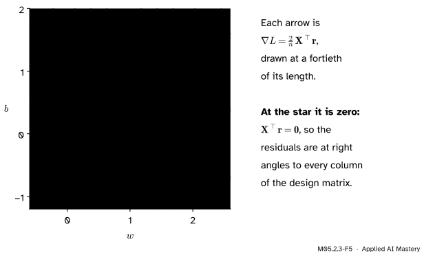
At a lowest point the gradient is zero, so \({\mat{X}\T\vect{r} = \vect{0}}\): the residual vector is at right angles to every column of \(\mat{X}\). Written out, \({\mat{X}\T\mat{X}\vect{w} = \mat{X}\T\vect{y}}\), the normal equations of least squares (M03.7.1).
M05.2.3-F5
The gradient \({\tfrac2n\mat{X}\T\vect{r}}\) at several points of the running loss. It vanishes only at the least-squares point \({(1.4, 0.5)}\), where the residuals are orthogonal to the columns of \(\mat{X}\).
NoteResult: the gradient of the mean log loss
For logistic regression, \({p_i = \sigma(z_i)}\) with scores \({\vect{z} = \mat{X}\vect{w}}\) and labels \({y_i \in \{0, 1\}}\). The mean log loss
\[
\begin{aligned}
\ell'(z) &= -y(1 - \sigma) + (1 - y)\sigma \\
&= \sigma - y = p - y .
\end{aligned}
\]
The score’s partial derivative is \({\pd{z_i}{w_j} = x_{ij}}\), as before, so \({\pd{L}{w_j} = \tfrac1n\sum_i (p_i - y_i)\,x_{ij}}\), which stacks into \({\tfrac1n\mat{X}\T(\vect{p} - \vect{y})}\). The pattern is the same as for least squares: the error at the output, \({\vect{p} - \vect{y}}\) in place of \(\vect{r}\), sent back through \({\mat{X}\T}\). Without the one half that some books put in front of squared errors, the factor is \({\tfrac2n}\) for squares and \({\tfrac1n}\) here.
Worked example
The running loss in matrix form. The design matrix has the column \({\vect{x} = (1, 2, 3, 4)}\) and a column of ones, and the parameter vector is \({\vect{w} = (w, b)}\). Two products do all the work:
the gradient of M04.10, now found without expanding the loss.
M05.2.3-F3
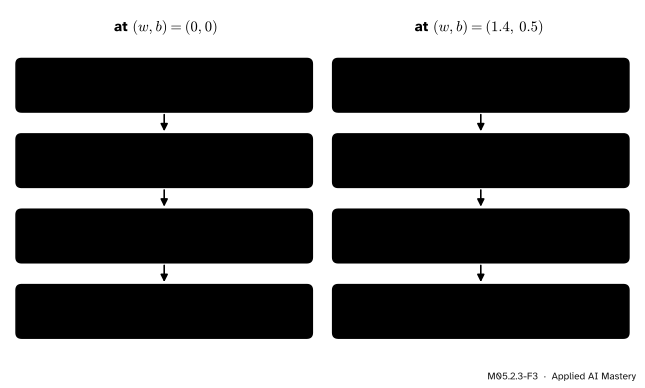
The gradient \({\tfrac2n\mat{X}\T\vect{r}}\) step by step, at the origin and at the least-squares point. At \({(1.4, 0.5)}\) the residuals cancel against both columns, and the gradient is zero.
At \({(1.4, 0.5)}\) the predictions are \({(1.9, 3.3, 4.7, 6.1)}\), so \({\vect{r} = (-0.1, 0.3, -0.3, 0.1)}\). Dotted with \(\vect{x}\): \({-0.1 + 0.6 - 0.9 + 0.4 = 0}\); with the ones: 0. The loss there is \({\tfrac14(0.01 + 0.09 + 0.09 + 0.01) = 0.05}\).
The log loss of the six students. The six students of ML01.6 studied \({1, 2, \dots, 6}\) hours, and those with 3, 5 and 6 hours passed: \({\vect{y} = (0, 0, 1, 0, 1, 1)}\). At \({(w, b) = (0, 0)}\) every score is 0 and every \({p_i = \tfrac12}\), so
Dotted with the hours: \({\tfrac12(1 + 2 - 3 + 4 - 5 - 6) = -3.5}\); with the ones: 0. Dividing by \({n = 6}\), \({\nabla L = (-0.583, 0)}\). The bias feels no pull because three students passed and three failed; the weight is pulled up, since the passes studied longer.
Code
From scratch: the gradient written as a loop over examples, exactly as in Step 2, and then as one line. They are checked on the running loss and on random data with five features.
import numpy as npdef mse_grad_loop(X, y, w): n, k = X.shape grad = np.zeros(k)for i inrange(n): # one example at a time r_i = X[i] @ w - y[i]for j inrange(k): # one weight at a time grad[j] +=2/ n * r_i * X[i, j]return graddef mse_grad(X, y, w):return2/len(y) * X.T @ (X @ w - y) # the whole gradient in one linex = np.array([1.0, 2.0, 3.0, 4.0])y = np.array([2.0, 3.0, 5.0, 6.0])X = np.column_stack([x, np.ones(4)]) # the design matrix: x, then onesprint("XtX =", (X.T @ X).tolist(), " Xty =", (X.T @ y).tolist())for w in ([0.0, 0.0], [1.0, 0.0], [1.4, 0.5]):# adding 0.0 turns a rounded -0.0 into 0.0print(w, mse_grad_loop(X, y, np.array(w)).round(10) +0.0, mse_grad(X, y, np.array(w)).round(10) +0.0)
The same two versions for the log loss, on the six students and on random data with five features and a bias.
def sigmoid(z):return1/ (1+ np.exp(-z))def log_loss_grad_loop(X, y, w): n, k = X.shape grad = np.zeros(k)for i inrange(n): p_i = sigmoid(X[i] @ w) grad += (p_i - y[i]) * X[i] / nreturn graddef log_loss_grad(X, y, w):return X.T @ (sigmoid(X @ w) - y) /len(y)hours = np.arange(1.0, 7.0)passed = np.array([0.0, 0.0, 1.0, 0.0, 1.0, 1.0])Xs = np.column_stack([hours, np.ones(6)])print("six students at (0, 0):", log_loss_grad(Xs, passed, np.zeros(2)).round(4))rng = np.random.default_rng(0)Xr = np.column_stack([rng.normal(size=(50, 5)), np.ones(50)]) # 50 examples, 5 features, a biasyr = (rng.random(50) <0.5).astype(float)wr = rng.normal(size=6)for name, loop, vec, target in (("mse", mse_grad_loop, mse_grad, Xr @ wr + rng.normal(size=50)), ("log loss", log_loss_grad_loop, log_loss_grad, yr)):print(name, "largest gap, loop vs one line:", np.abs(loop(Xr, target, wr) - vec(Xr, target, wr)).max())
six students at (0, 0): [-0.5833  0.    ]
mse largest gap, loop vs one line: 1.1102230246251565e-16
log loss largest gap, loop vs one line: 1.1102230246251565e-16
Both versions agree to rounding (the last digits may differ from machine to machine). The one-line version hands the double loop to NumPy’s compiled matrix product, which is what makes large models practical. Whether either is correct is the question of the next lesson.
Explore
This module’s interactive lives in lesson M05.2.2. Choose the running loss there: its gradient arrow is the \({\tfrac2n\mat{X}\T\vect{r}}\) of this lesson, and the tangent plane it defines predicts how a small step in \((w, b)\) changes the loss.
Pitfalls
M05.2.3-F4
Wrong beside right. Defining the residual as \({y - \hat y}\) but keeping the formula \({\tfrac2n\mat{X}\T\vect{r}}\) flips the gradient. The same descent step of 0.03 then raises the loss from 18.5 to 41.6 instead of lowering it to 4.6.
“The residual is target minus prediction, and the formula stays the same.”
Either convention works if it is carried through, but the sign of the gradient depends on it. With \({\vect{r} = \vect{y} - \mat{X}\vect{w}}\) the gradient is \({-\tfrac2n\mat{X}\T\vect{r}}\). Mixing the two sends descent uphill, as in the figure. A quick test: at a point far from the fit, one small step against the gradient must lower the loss.
“The sum and the mean have the same gradient.”
They point the same way, but the sum’s gradient is \(n\) times longer. Code that sums the loss over a batch but was tuned with a mean needs a learning rate \(n\) times smaller, and changing the batch size silently changes the step. State which one the loss is, and keep the factor in the gradient.
“X @ r and X.T @ r are the same thing.”
\(\mat{X}\) is \({n \times (d + 1)}\) and \(\vect{r}\) has \(n\) entries, so only \({\mat{X}\T\vect{r}}\) fits. When \({n = d + 1}\) both run without an error and give different numbers. Check that the gradient has the shape of the weights before trusting it.
Check yourself
Recall
1. What is \({\pd{L}{w_j}}\) for \({L = \tfrac1n\sum_i r_i^2}\) with \({r_i = \vect{w}\T\vect{x}_i + b - y_i}\)?
Show answer
\({\tfrac2n\sum_i r_i\,x_{ij}}\): the average of twice the residual times feature \(j\).
2. How does the bias enter the design matrix?
Show answer
As a column of ones. The bias is then the last entry of \(\vect{w}\), and its partial derivative is \({\tfrac2n\sum_i r_i}\), the dot product of that column with \(\vect{r}\).
3. Write the gradient of the mean squared error in matrix form, and give its shape.
Show answer
\({\tfrac2n\mat{X}\T(\mat{X}\vect{w} - \vect{y})}\), of shape \({(d + 1) \times 1}\), the shape of \(\vect{w}\).
4. What is the derivative of one example’s log loss with respect to its score \(z\)?
Show answer
\({p - y}\), the predicted probability minus the label.
5. What does \({\mat{X}\T\vect{r} = \vect{0}}\) say about the residuals at the least-squares solution?
Show answer
They are at right angles to every column of \(\mat{X}\); written out, these are the normal equations \({\mat{X}\T\mat{X}\vect{w} = \mat{X}\T\vect{y}}\).
Exercises
1.★ Find the gradient of the running loss at \({(w, b) = (2, 0)}\) from \({\tfrac2n\mat{X}\T\vect{r}}\), and check it against \({(15w + 5b - 23.5,\; 5w + 2b - 8)}\).
Show solution
The predictions are \({2\vect{x} = (2, 4, 6, 8)}\), so \({\vect{r} = (0, 1, 1, 2)}\). Dotted with \(\vect{x}\): \({0 + 2 + 3 + 8 = 13}\); with the ones: 4. Times \({\tfrac24}\): \({(6.5, 2)}\). The formula gives \({30 - 23.5 = 6.5}\) and \({10 - 8 = 2}\).
2.★★ A weighted loss gives example \(i\) a weight \({c_i > 0}\): \({L = \tfrac1n\sum_i c_i r_i^2}\). Find its gradient in matrix form.
Show solution
By the chain rule \({\pd{}{w_j}(c_ir_i^2) = 2c_ir_ix_{ij}}\), so \({\pd{L}{w_j} = \tfrac2n\sum_i x_{ij}(c_ir_i)}\). Write \({\mat{C}}\) for the diagonal matrix with the \(c_i\) on its diagonal; then \({c_ir_i}\) is entry \(i\) of \({\mat{C}\vect{r}}\), and the gradient is \({\tfrac2n\mat{X}\T\mat{C}\vect{r}}\). With every \({c_i = 1}\) it is the ordinary result.
3.★★★ Show that at \({\vect{w} = \vect{0}}\) the log-loss gradient in the bias is \({\tfrac12 - \bar y}\), where \({\bar y}\) is the fraction of positive labels, and say what a gradient step on \(b\) alone then does.
Show solution
At \({\vect{w} = \vect{0}}\) every score is 0, so every \({p_i = \sigma(0) = \tfrac12}\). The bias column is all ones, so \({\pd{L}{b} = \tfrac1n\sum_i (\tfrac12 - y_i) = \tfrac12 - \bar y}\). If more than half the labels are 1, this is negative, so a step against the gradient raises \(b\) and every predicted probability towards \({\bar y}\); if fewer than half, it lowers them. For the six students \({\bar y = \tfrac12}\) and the pull is zero, as in the worked example.
Summary card
Every weight’s slope is residual times feature, averaged: together, Xᵀr.
M05.2.3-F1
Residuals in, gradient out.
Mean squared error.\({\nabla L = \tfrac2n\mat{X}\T(\mat{X}\vect{w} - \vect{y})}\).
Mean log loss.\({\nabla L = \tfrac1n\mat{X}\T(\vect{p} - \vect{y})}\), from \({\ell'(z) = p - y}\).
Bias. A column of ones in \(\mat{X}\).
Shapes.\({(d + 1) \times n}\) times \({n \times 1}\): one entry per weight.
Lowest point.\({\mat{X}\T\vect{r} = \vect{0}}\), the normal equations.
Sources and next steps
Sources. Each was opened and checked against this lesson on 15 November 2026.
Marc Peter Deisenroth, A. Aldo Faisal and Cheng Soon Ong, Mathematics for Machine Learning, Example 5.11 in Section 5.3: the gradient of the least-squares loss \({\norm{\vect{y} - \mat{\Phi}\vect{\theta}}^2}\) by the chain rule, \({-2\vect{e}\T\mat{\Phi}}\) with the error \({\vect{e} = \vect{y} - \mat{\Phi}\vect{\theta}}\) (Equation 5.83), written as a row and with the opposite sign of residual.
Tengyu Ma and Andrew Ng, CS229 Lecture Notes, Stanford University. Section 1.2.2 sets the derivatives of the least-squares cost to zero and obtains the normal equations \({\mat{X}\T\mat{X}\vect{\theta} = \mat{X}\T\vect{y}}\); Section 2.1 differentiates the log-likelihood of logistic regression for one example, \({(y - h_\theta(x))\,x_j}\) (Equation 2.2), using \({g'(z) = g(z)(1 - g(z))}\). They maximise the likelihood, so their sign is the opposite of ours.