Partial derivatives and the gradient in n variables
Freeze every input but one and a function of many inputs becomes an ordinary curve with an ordinary slope. Collect those slopes, one per input, into a column: the gradient. Worked on a function of three inputs, the norm, a linear score and the logistic model.
M05.2.1L2 Intermediate25 minIn review (what this means)
The maths and code on this page are checked by automated tests on every change, but an independent reader has not signed it off yet. Spot a mistake or a confusing step? Tell us.
Define the partial derivative of a function of n inputs as the slope of a slice in which every other input is held fixed.
Compute partial derivatives term by term, treating the inputs that do not move as constants.
Assemble the gradient as a column with the shape of the input, and state the gradients of the dot product with a fixed vector, the squared norm and the norm.
Differentiate the logistic model with respect to its weights by the chain rule and the slope of the sigmoid.
Estimate a gradient with central differences in each coordinate, 2n evaluations, and check it against the hand result.
The question
A model with three weights has a loss that depends on all three at once. A real network has millions. Training needs, for every single weight, an answer to one question: if this weight alone moves a little, how fast does the loss change? M04.10 answered it for two inputs. What is the answer for \(n\) inputs, and what shape does the collection of answers have?
Intuition
A function of three inputs cannot be drawn as a surface: its graph would need four dimensions. But you never need the whole graph to find one slope. Hold two inputs fixed, let only the third move, and what is left is an ordinary function of one variable, a curve you can draw, with an ordinary slope at the point. That slope is a partial derivative.
Do it once for each input and you have \(n\) slopes. Stack them in the order of the inputs and you have the gradient, a column with one entry per input, the same shape as the point itself.
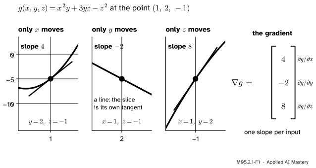
M05.2.1-F1
One function of three inputs, three slices through the same point. In each slice two inputs are held at their values and one moves. The three slopes, in the order of the inputs, make the gradient \({(4, -2, 8)}\).
Nothing here is new in kind. Each slice is a function of one variable, and its slope is the derivative of M04.2. What is new is the bookkeeping: \(n\) slices, \(n\) slopes, and one column that holds them all. That column is what gradient descent subtracts from the weights at every step.
Build it up
Step 1. One slice, from the definition. Take \({g(x, y, z) = x^2y + 3yz - z^2}\), the function \({x^2y + 3y}\) of M04.10.2 with a third input added, at the point \({(1, 2, -1)}\). There \({g = 2 - 6 - 1 = -5}\). Hold \({y = 2}\) and \({z = -1}\) and let \(x\) move by \(h\):
The difference quotient is \({(4h + 2h^2)/h = 4 + 2h}\), which tends to 4 as \(h\) tends to 0. So the partial derivative of \(g\) in \(x\) at the point is 4: the slope of the first slice in the figure.
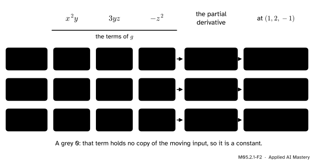
Step 2. Every slice, by the rules. The limit is the definition, but no one computes it each time. In a slice the held inputs are just numbers, so the rules of M04.3 apply with them treated as constants. Go term by term. In \({x^2y}\) the factor \(y\) is a constant multiple, so its derivative in \(x\) is \({2xy}\); \({3yz}\) and \({-z^2}\) contain no \(x\) at all, so they are constants with derivative 0.
M05.2.1-F2
Term by term. Each row lets one input move and treats the others as constants. A term that does not contain the moving input is a constant and contributes 0.
At \({(1, 2, -1)}\) they are \({2 \cdot 1 \cdot 2 = 4}\), \({1 - 3 = -2}\) and \({6 + 2 = 8}\). The middle one is the slope of a straight line: with \(x\) and \(z\) held, \(g\) is \({-2y - 1}\), and a line is its own tangent.
Step 3. Stack them. The point is a column of three numbers. Write the three slopes as a column in the same order, and you have the gradient at the point:
Read it entry by entry: moving \(z\) alone changes \(g\) twice as fast as moving \(x\) alone, and moving \(y\) alone makes it fall.
The formal statement
NoteDefinitions: partial derivative and gradient
Let \({f : \R^n \to \R}\) and let \(\vect{e}_i\) be the \(i\)-th standard basis vector. The partial derivative of \(f\) in its \(i\)-th input at \(\vect{a}\) is
Adding \({h\,\vect{e}_i}\) changes input \(i\) by \(h\) and leaves the others alone, so the quotient is the slope of a secant of the slice through \(\vect{a}\) along axis \(i\). The gradient has the shape of its argument: \(n\) inputs, \(n\) entries. Mathematics for Machine Learning writes the same numbers as a row, the \({1 \times n}\) Jacobian; this course writes a column and keeps rows for Jacobians (M05.4).
Three gradients come up all through machine learning. Each is derived from the definition of a partial derivative and the one-variable rules.
A dot product with a fixed vector. Let \({f(\vect{x}) = \vect{w}\T\vect{x} = w_1x_1 + \dots + w_nx_n}\). In the partial derivative in \(x_j\), every term except \({w_jx_j}\) is a constant, so \({\pd{f}{x_j} = w_j}\). All \(n\) entries together:
\[
\nabla(\vect{w}\T\vect{x}) = \vect{w} .
\]
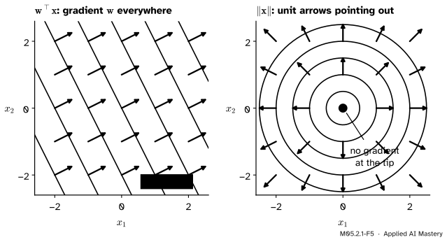
The same arrow at every point: a linear score climbs equally fast everywhere.
The squared norm.\({\norm{\vect{x}}^2 = x_1^2 + \dots + x_n^2}\), and only the term \({x_j^2}\) holds \(x_j\), so \({\pd{}{x_j}\norm{\vect{x}}^2 = 2x_j}\) and \({\nabla\norm{\vect{x}}^2 = 2\vect{x}}\).
The norm.\({\norm{\vect{x}} = s^{1/2}}\) with \({s = x_1^2 + \dots + x_n^2}\). By the chain rule (M04.3.4), with \({\pd{s}{x_j} = 2x_j}\),
so \({\nabla\norm{\vect{x}} = \vect{x}/\norm{\vect{x}}}\) for \({\vect{x} \neq \vect{0}}\): a vector of length 1 pointing straight away from the origin. At \({\vect{x} = \vect{0}}\) the formula divides by zero, and the gradient does not exist.
M05.2.1-F5
Gradients as arrows on the plane. Left: for \({\vect{w}\T\vect{x}}\) the gradient is \(\vect{w}\) at every point. Right: for \({\norm{\vect{x}}}\) it has length 1 and points outwards; at the origin, the tip of the cone, there is none.
Go deeper: why the norm has no partial derivatives at the origin
Along axis 1 through the origin the norm is \({\norm{t\,\vect{e}_1} = \abs{t}}\). The difference quotient of the definition is \({\abs{h}/h}\), which is \(+1\) for every positive \(h\) and \(-1\) for every negative \(h\). The two one-sided limits differ, so the limit does not exist: the slice has a corner, like the absolute value of M04.2.3. Every axis gives the same corner, so not one partial derivative exists at \(\vect{0}\). The squared norm has no such trouble: its slice is \(t^2\), with slope 0.
Worked example
The norm at \({\vect{x} = (1, 2, 2)}\). Here \({\norm{\vect{x}} = \sqrt{1 + 4 + 4} = 3}\), so \({\nabla\norm{\vect{x}} = (1, 2, 2)/3 = (\tfrac13, \tfrac23, \tfrac23)}\). Its length is \({\sqrt{1 + 4 + 4}/3 = 1}\), as the formula promised.
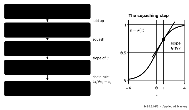
The logistic model in its weights. The logistic model of ML01.6 outputs \({p = \sigma(\vect{w}\T\vect{x} + b)}\), where \({\sigma(z) = 1/(1 + e^{-z})}\). For training, the inputs \(\vect{x}\) are fixed data and the weights move, so take the gradient in \(\vect{w}\), written \({\nabla_{\vect{w}}}\). Write \({z = \vect{w}\T\vect{x} + b}\). By the chain rule,
The slope of the sigmoid is \({\sigma'(z) = \sigma(z)(1 - \sigma(z)) = p(1 - p)}\) (M04.3.3), and \({\pd{z}{w_j} = x_j}\) by the dot-product result above. So
Now numbers: \({\vect{w} = (0.5, -1, 2)}\), \({b = 0}\) and \({\vect{x} = (2, 1, 0.5)}\).
M05.2.1-F3
The logistic model’s gradient in its weights, one step at a time. The only slope that needs any work is the sigmoid’s, at \({z = 1}\); the chain rule multiplies it by each input.
The score is \({z = 0.5 \cdot 2 - 1 \cdot 1 + 2 \cdot 0.5 = 1}\), so \({p = \sigma(1) \approx 0.731}\) and \({p(1 - p) \approx 0.731 \times 0.269 \approx 0.197}\). Then
The weight on the largest input moves the output fastest. And since \({p(1 - p)}\) is at most \({\tfrac14}\), reached at \({p = \tfrac12}\), the output is most sensitive to its weights when the model is least sure.
Code
From scratch first: a central difference (M04.2.4) in each coordinate in turn, the others held. A counter records how often the function is called.
import numpy as npcalls =0def numerical_gradient(f, a, h=1e-5):"""Central difference along each axis: 2 evaluations per input, 2n in all.""" a = np.asarray(a, dtype=float) grad = np.zeros_like(a)for i inrange(a.size): step = np.zeros_like(a) step[i] = h # move input i only grad[i] = (f(a + step) - f(a - step)) / (2* h)return graddef g(v):global calls calls +=1 x, y, z = vreturn x**2* y +3* y * z - z**2def grad_g(v): x, y, z = vreturn np.array([2* x * y, x**2+3* z, 3* y -2* z])a = np.array([1.0, 2.0, -1.0])print("by hand: ", grad_g(a))print("numerical:", numerical_gradient(g, a).round(6), " calls:", calls)
The six calls are the \({2n}\) of the method with \({n = 3}\). Now the three gradients of the formal statement and the logistic model, each against the same numerical routine. The dot product is tried with a thousand inputs, to see the cost grow.
def sigmoid(z):return1/ (1+ np.exp(-z))x_in = np.array([2.0, 1.0, 0.5])p =lambda w: sigmoid(w @ x_in) # b = 0w0 = np.array([0.5, -1.0, 2.0])pw = p(w0)print("logistic, by hand: ", (pw * (1- pw) * x_in).round(3))print("logistic, numerical:", numerical_gradient(p, w0).round(3))v = np.array([1.0, 2.0, 2.0])print("norm at (1, 2, 2):", numerical_gradient(np.linalg.norm, v).round(4))rng = np.random.default_rng(0)w_big = rng.normal(size=1000)def score(x): # w.x with a call counterglobal calls calls +=1return w_big @ xcalls =0grad_dot = numerical_gradient(score, rng.normal(size=1000))print("w.x with n = 1000: largest error", np.abs(grad_dot - w_big).max(), " calls:", calls)
logistic, by hand:   [0.393 0.197 0.098]
logistic, numerical: [0.393 0.197 0.098]
norm at (1, 2, 2): [0.3333 0.6667 0.6667]
w.x with n = 1000: largest error 5.110081247039489e-10  calls: 2000
Every numerical gradient matches its hand formula. For the dot product with \({n = 1000}\) the routine needed 2,000 calls to rebuild a vector we already knew; M05.2.4 returns to that cost. SciPy’s scipy.differentiate.jacobian does the same job with a more careful difference scheme. Given a function with one output it returns the gradient as a flat array, one entry per input.
This module’s interactive, the linear-model checker, lives in the next lesson. It puts the gradient to work: the arrow from this lesson predicts how far the function rises for any small step.
Pitfalls
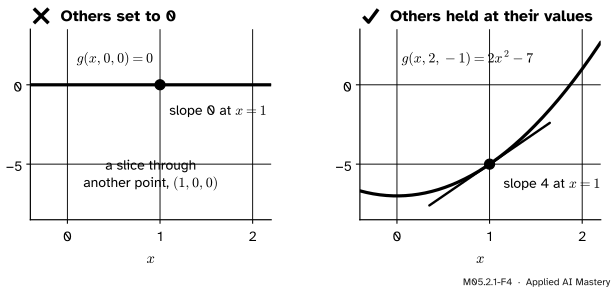
M05.2.1-F4
Wrong beside right, for \({\pd{g}{x}}\) at \({(1, 2, -1)}\). Setting the other inputs to 0 slices through a different point and gives slope 0. Holding them at 2 and \(-1\) gives the true slope, 4.
“Holding the other inputs fixed means setting them to zero.”
They are held at their values at the point. In \({\pd{}{x}(x^2y) = 2xy}\) the \(y\) stays a letter while you differentiate, and only then takes its value, 2. Putting \({y = 0}\) first slices through \({(1, 0, 0)}\), a different point, where the slope in \(x\) is 0, not 4.
“A gradient is a row, or any shape that holds the numbers.”
In this course the gradient has the shape of its argument. A weight vector of shape (5,) has a gradient of shape (5,), so the update w - lr * grad lines up entry by entry. Books that write gradients as rows, such as Mathematics for Machine Learning, hold the same numbers; check which convention a formula uses before you multiply it by a matrix.
“Every formula for a gradient works everywhere.”
\({\vect{x}/\norm{\vect{x}}}\) divides by zero at the origin, where the norm has a corner and no gradient. In NumPy, x / np.linalg.norm(x) at zero returns nan and a warning. Code that uses the norm itself as a penalty must handle that point, or use the squared norm, whose gradient \({2\vect{x}}\) exists everywhere.
Check yourself
Recall
1. In words, what is \({\pd{f}{x_i}(\vect{a})}\)?
Show answer
The slope at \(\vect{a}\) of the slice in which every input except \(x_i\) is held at its value at \(\vect{a}\): the limit of \({(f(\vect{a} + h\vect{e}_i) - f(\vect{a}))/h}\).
2. What shape does the gradient of a function of \({\vect{x} \in \R^n}\) have here?
Show answer
The shape of its argument: a column of \(n\) entries, the \(i\)-th being \({\pd{f}{x_i}}\).
3. What is \({\nabla(\vect{w}\T\vect{x})}\), and what is \({\nabla\norm{\vect{x}}^2}\)?
Show answer
\(\vect{w}\), the same at every point, and \({2\vect{x}}\).
4. Where does \({\nabla\norm{\vect{x}}}\) fail to exist, and why?
Show answer
At \({\vect{x} = \vect{0}}\). Along each axis the norm is \({\abs{t}}\), which has a corner at 0; the formula \({\vect{x}/\norm{\vect{x}}}\) divides by zero there.
5. How many evaluations of \(f\) does a central-difference gradient in \(n\) variables take?
Show answer
\({2n}\): one step forwards and one backwards along each of the \(n\) axes.
Exercises
1.★ Find the gradient of \({f(x, y, z) = xe^{yz}}\) and evaluate it at \({(2, 0, 3)}\).
Show solution
Term by term with the other inputs as constants: \({\pd{f}{x} = e^{yz}}\); in \(y\), by the chain rule, \({\pd{f}{y} = xz\,e^{yz}}\); in \(z\), \({\pd{f}{z} = xy\,e^{yz}}\). At \({(2, 0, 3)}\) the exponent is \({yz = 0}\), so \({e^{yz} = 1}\) and
2.★★ For a fixed vector \(\vect{c}\), find the gradient of \({f(\vect{x}) = \norm{\vect{x} - \vect{c}}^2}\), and say where it is zero.
Show solution
\({f = (x_1 - c_1)^2 + \dots + (x_n - c_n)^2}\). Only the \(j\)-th term holds \(x_j\), and its derivative is \({2(x_j - c_j)}\) by the chain rule. So \({\nabla f = 2(\vect{x} - \vect{c})}\). It is zero only at \({\vect{x} = \vect{c}}\), where \(f\) takes its lowest value, 0. The gradient points straight away from \(\vect{c}\), so a step against it heads straight back.
3.★★★ The softplus \({\operatorname{sp}(z) = \ln(1 + e^z)}\) has derivative \(\sigma(z)\). Find the gradient in \(\vect{w}\) of \({f(\vect{w}) = \operatorname{sp}(\vect{w}\T\vect{x})}\), and evaluate it for the \(\vect{w}\) and \(\vect{x}\) of the worked example.
Show solution
Write \({z = \vect{w}\T\vect{x}}\). By the chain rule \({\pd{f}{w_j} = \operatorname{sp}'(z)\,\pd{z}{w_j} = \sigma(z)\,x_j}\), so \({\nabla_{\vect{w}} f = \sigma(\vect{w}\T\vect{x})\,\vect{x}}\). In the worked example \({z = 1}\) and \({\sigma(1) \approx 0.731}\), so
(The derivative of \({\ln(1 + e^z)}\) is \({e^z/(1 + e^z) = 1/(e^{-z} + 1) = \sigma(z)}\), dividing top and bottom by \(e^z\).)
Summary card
A gradient is one slope per input, stacked like the input.
M05.2.1-F1
Three slices, three slopes, one column.
Partial derivative.\({\pd{f}{x_i}}\): the slope along axis \(i\), the other inputs held.
Gradient. The column of all \(n\) partial derivatives, shaped like \(\vect{x}\).
Three to know.\({\nabla(\vect{w}\T\vect{x}) = \vect{w}}\), \({\nabla\norm{\vect{x}}^2 = 2\vect{x}}\), \({\nabla\norm{\vect{x}} = \vect{x}/\norm{\vect{x}}}\) off the origin.
Numerically. Central differences on each axis, \({2n}\) evaluations.
Sources and next steps
Sources. Each was opened and checked against this lesson on 15 November 2026.
Gilbert Strang and Edwin Herman, Calculus Volume 3 (OpenStax), Section 4.3: the partial derivatives of a function of two variables as limits (Equations 4.12 and 4.13), and the subsection “Functions of More Than Two Variables”, with the three partial derivatives of \({f(x, y, z)}\) as limits (Equations 4.14 to 4.16).
Marc Peter Deisenroth, A. Aldo Faisal and Cheng Soon Ong, Mathematics for Machine Learning, Section 5.2: Definition 5.5 (partial derivatives of \({f : \R^n \to \R}\), “varying one variable at a time and keeping the others constant”), Equation 5.40 (the gradient, which the book writes as a \({1 \times n}\) row) and the remark “Gradient as a Row Vector”.
SciPy 1.18 reference, scipy.differentiate.jacobian: the signature and defaults (order=8, initial_step=0.5), and its Rosenbrock example, where a function with one output and three inputs gives df of shape (3,).