A vector field puts an arrow at every point of the plane, and a flow line is the path that always moves along the arrow under its feet. Draw fields by hand, solve their flow lines exactly and by Euler steps, and see gradient descent as one such path.
M05.10.1L2 Intermediate25 minIn review (what this means)
The maths and code on this page are checked by automated tests on every change, but an independent reader has not signed it off yet. Spot a mistake or a confusing step? Tell us.
Draw a vector field from R^2 to R^2 by hand on a grid, and read off where it points out, in or round.
Solve the flow-line equation x’(t) = F(x(t)) exactly for the source (x, y), the rotation (-y, x) and gradient descent on the running bowl.
Trace a flow line by Euler steps, and prove that on the rotation field each step multiplies the distance from the origin by the square root of 1 + (Delta t)^2.
Explain why gradient descent is Euler’s method on the field -grad L, and why simultaneous descent and ascent on the game x y circles instead of settling.
The question
A loss gives a gradient at every setting of the weights, and gradient descent moves the weights a little way along the arrow under its feet, again and again. What path does that make? And when two players each follow their own arrow, as the two networks of a GAN do, why can the pair circle for ever instead of settling down?
Intuition
A vector field on the plane attaches an arrow to every point. Wind on a weather map is one: at each place, an arrow says which way the air moves and how fast. The gradient of a function is another: at each point it says which way is steepest uphill.
Drop a cork into the wind and it drifts, always moving along the arrow at its current spot. Its path is a flow line of the field.
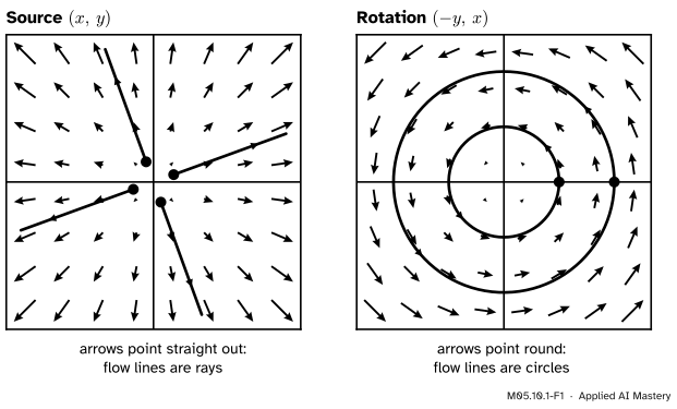
M05.10.1-F1
Two running fields of the module. The source\({(x, y)}\) points away from the origin, so a cork runs straight out along a ray. The rotation\({(-y, x)}\) points round the origin, so a cork goes round a circle and comes back to where it started.
The two pictures already show the two behaviours that the rest of the module measures. Arrows that spread out push things apart: that will be the divergence (lesson M05.10.3). Arrows that turn round carry things in loops: that will be the curl (lesson M05.10.4). This lesson is about the arrows themselves and the paths they make.
Build it up
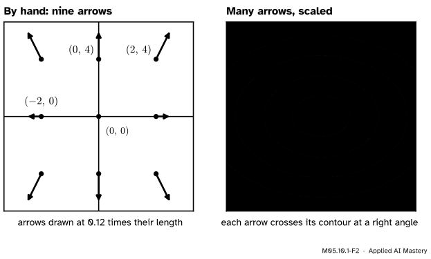
Step 1. An arrow at each point. A vector field on the plane is a rule \({\vect{F}(x, y) = (P(x, y),\, Q(x, y))}\): two functions, one for each component of the arrow. To draw it, pick points, work out the arrow there and draw it with its tail, or its middle, at the point. At \({(1, 0.5)}\) the source gives \({(1, 0.5)}\), the rotation gives \({(-0.5, 1)}\), and the gradient field \({(2x, 4y)}\) of the running bowl \({f(x, y) = x^2 + 2y^2}\) gives \({(2, 2)}\).
Step 2. Scale the arrows together. True lengths overlap and clutter the page, so every arrow is drawn shrunk by the same factor. Lengths then stay in proportion: twice as long still means twice as strong.
M05.10.1-F2
The gradient field of the running bowl. By hand, nine arrows are enough to see the pattern; a computer draws many, scaled together. Each arrow is perpendicular to the contour through its point.
Step 3. A path that follows the arrows. A flow line is a path \({\vect{x}(t)}\) whose velocity at every moment is the arrow where it is:
\[
\vect{x}'(t) = \vect{F}(\vect{x}(t)) .
\]
This is a system of two differential equations, \({x' = P(x, y)}\) and \({y' = Q(x, y)}\), of exactly the kind M04.9 solved for one unknown. A starting point picks out one flow line.
Step 4. When no formula solves it, take small steps. Euler’s method from M04.9.4 works unchanged with vectors: from \({\vect{x}_k}\), follow the arrow there for a short time \({\Delta t}\), then look again.
A vector field on a region \({D \subseteq \R^2}\) is a function \({\vect{F} : D \to \R^2}\), written \({\vect{F} = (P, Q)}\). A flow line (or integral curve) of \(\vect{F}\) is a differentiable path \({\vect{x}(t)}\) in \(D\) with \({\vect{x}'(t) = \vect{F}(\vect{x}(t))}\) for every \(t\). A field \({\vect{F} = \nabla f}\) is a gradient field, and \(f\) is its potential.
When \(P\) and \(Q\) have continuous partial derivatives, exactly one flow line passes through each starting point, so flow lines never cross. That uniqueness theorem is proved in M12.1; here we solve three cases by hand.
The source \({(x, y)}\). The equations are \({x' = x}\) and \({y' = y}\). They do not interact, and each is the growth equation of M04.9.2, so from \({(x_0, y_0)}\)
The point is always \({e^t}\) times its start: it runs straight out along a ray, and its distance from the origin grows exponentially.
The rotation \({(-y, x)}\). Now the equations are coupled: \({x' = -y}\) and \({y' = x}\). First show that the distance from the origin cannot change. Differentiate its square with the chain rule:
So the path stays on the circle through its start. Try \({x = r_0\cos(t + \varphi)}\) and \({y = r_0\sin(t + \varphi)}\): then \({x' = -r_0\sin(t + \varphi) = -y}\) and \({y' = r_0\cos(t + \varphi) = x}\), as required. The point goes anticlockwise round the circle at unit angular speed and returns after time \({2\pi}\).
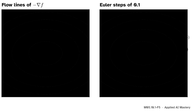
Gradient descent on the bowl. Descent follows the field \({-\nabla f = (-2x, -4y)}\). Again the equations separate, giving \({x = x_0e^{-2t}}\) and \({y = y_0e^{-4t}}\). Since \({e^{-4t} = (e^{-2t})^2}\), every flow line is part of the parabola \({y = y_0\,(x / x_0)^2}\): from \({(1, 1)}\) it is \({y = x^2}\).
M05.10.1-F5
Gradient descent on the bowl. Left: the exact flow lines are parabolas, and they enter the minimum along the flat \({x}\)-direction, where the bowl curves least. Right: gradient descent with learning rate 0.1 is a chain of Euler steps that stays close to the flow line.
Gradient descent is Euler’s method. Put \({\vect{F} = -\nabla L}\) into Euler’s step:
That is the gradient-descent update with learning rate \({\eta = \Delta t}\), as M04.9.4 found in one variable. On the bowl from \({(1, 1)}\) with \({\eta = 0.1}\), the first step is \({(1, 1) - 0.1\,(2, 4)} = {(0.8, 0.6)}\) and the second \({(0.8, 0.6) - 0.1\,(1.6, 2.4)} = {(0.64, 0.36)}\).
Go deeper: why each coordinate of the bowl's descent shrinks by its own factor
In each step the \({x}\)-coordinate is multiplied by \({1 - 2\eta}\) and the \({y}\)-coordinate by \({1 - 4\eta}\), because the gradient’s components are \({2x}\) and \({4y}\). With \({\eta = 0.1}\) the factors are 0.8 and 0.6, so after \(k\) steps the point is \({(0.8^k, 0.6^k)}\). The exact flow multiplies by \({e^{-0.2} \approx 0.819}\) and \({e^{-0.4} \approx 0.670}\) per unit of 0.1 in time: close, which is why the chain hugs the parabola. If \({\eta > 0.5}\), then \({1 - 4\eta < -1}\) and the \(y\)-coordinate flips sign and grows: the step-size limit of M04.9.4, now set by the steeper direction.
Worked example
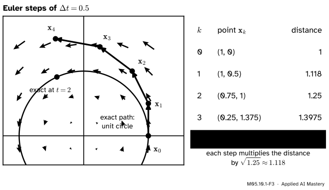
Four Euler steps round the rotation. Start at \({\vect{x}_0 = (1, 0)}\) on the rotation field and take steps of \({\Delta t = 0.5}\). The exact flow line is the unit circle. Each step adds half the arrow \({(-y, x)}\) at the current point.
The worked example as a trace. The exact path stays on the unit circle; Euler’s chain spirals outwards, ending at distance 1.5625 when the true point \({(\cos 2, \sin 2)}\) is at distance 1.
After time \({4 \times 0.5 = 2}\) the exact point is \({(\cos 2, \sin 2) \approx (-0.416, 0.909)}\), on the circle. Euler’s point is at distance \({\sqrt{0.4375^2 + 1.5^2} = 1.5625}\). The distances in the table go 1, 1.118, 1.25, 1.398, 1.5625: each is the one before times \({\sqrt{1.25}}\).
Why. For one step from \({(x, y)}\) the new point is \({(x - \Delta t\,y,\; y + \Delta t\,x)}\). Its squared distance from the origin is
because the cross terms \({-2\Delta t\,xy}\) and \({+2\Delta t\,xy}\) cancel. So every step multiplies the distance by \({\sqrt{1 + \Delta t^2}}\), here \({\sqrt{1.25} \approx 1.118}\). However small the step, Euler’s method spirals out of the circle; a smaller step only slows the spiral.
The same field in a game. Two players share the payoff \({f(x, y) = xy}\): the first picks \(x\) and wants \(f\) small, the second picks \(y\) and wants it large. Simultaneous gradient play moves \({x}\) down its partial derivative and \({y}\) up its own:
That is the rotation field. The exact flow circles the balance point \({(0, 0)}\) for ever, and the discrete steps a computer takes spiral away from it, as the trace shows. Balduzzi and colleagues use this example (with a matrix in place of the single number) to explain why gradient play on games such as GANs can cycle.
Code
Euler’s method for a field takes three lines. Then the same flow lines with SciPy’s general solver, which adapts its steps to meet an error tolerance.
import numpy as npdef rotation(p): x, y = preturn np.array([-y, x])def euler(field, start, dt, steps):"""Euler steps x_{k+1} = x_k + dt F(x_k); returns all the points as rows.""" points = [np.asarray(start, dtype=float)]for _ inrange(steps): points.append(points[-1] + dt * field(points[-1]))return np.array(points)trace = euler(rotation, (1.0, 0.0), 0.5, 4)print(trace)print("distances:", np.round(np.hypot(trace[:, 0], trace[:, 1]), 4))# Gradient descent on the bowl f = x^2 + 2y^2 is Euler's method on -grad f.descent =lambda p: -np.array([2* p[0], 4* p[1]])print("descent:", euler(descent, (1.0, 1.0), 0.1, 2)[1:])
Now scipy.integrate.solve_ivp, which wants the right-hand side as fun(t, y) with the time first. Its answer sol.y has one row per coordinate and one column per stored time.
from scipy.integrate import solve_ivpsol = solve_ivp(lambda t, p: rotation(p), (0, 2* np.pi), [1.0, 0.0], rtol=1e-10, atol=1e-12, t_eval=[2.0, 2* np.pi])print("at t = 2: ", np.round(sol.y[:, 0], 4), " exact:", np.round([np.cos(2), np.sin(2)], 4))print("at t = 2pi:", np.round(sol.y[:, 1], 6))src = solve_ivp(lambda t, p: p, (0, 1), [0.5, 0.25], rtol=1e-10, atol=1e-12)print("source after t = 1:", np.round(src.y[:, -1], 4), " = e times the start")
at t = 2:   [-0.4161  0.9093]   exact: [-0.4161  0.9093]
at t = 2pi: [1. 0.]
source after t = 1: [1.3591 0.6796]  = e times the start
The solver closes the circle to within \({10^{-8}}\) after one full turn, where four Euler steps had already drifted 0.56 too far from the origin. The difference is the size of the steps it takes and the higher-order method it uses, not a different idea: it still follows the arrows.
Frontier note: the score field of a density
For a probability density \({p}\) on the plane, the field \({\nabla \log p}\) is called its score. It points uphill in probability. For the standard Gaussian, \({\log p = -(x^2 + y^2)/2 + \text{const}}\), so the score is \({-(x, y)}\): the source reversed, every arrow pointing at the mode. Song and Ermon (2019) train a network to estimate the score of a data distribution from samples and then generate new samples by following it with small noisy steps (Langevin dynamics). Diffusion models (DL07, M12.6) are built on this idea: learn a vector field, then follow its flow lines.
Explore
This module’s interactive, the field explorer, lives in lesson M05.10.3. Choose the rotation there, click near the centre to drop a particle and watch its Euler path spiral slowly outwards; set the step slider larger and the spiral opens up, as the worked example predicts.
Pitfalls
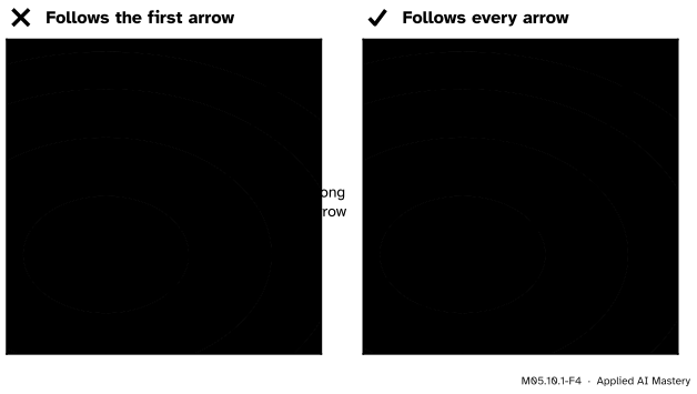
M05.10.1-F4
Wrong beside right. A flow line is not the straight line along the first arrow: that line misses the minimum by about 0.45. The true path turns as the arrows turn and arrives exactly.
“The path goes where the first arrow points.”
Only for an instant. From \({(1, 1)}\) the descent arrow is \({(-2, -4)}\), and the straight line along it comes no nearer the minimum than \({(0.4, -0.2)}\), about 0.45 away. The flow line asks the field again at every point, so it turns towards the flatter \(x\)-direction and reaches \({(0, 0)}\). A long gradient step makes the same mistake, which is why the learning rate must be small.
“With a small enough step, Euler’s path round a circle closes.”
It never does. Each step multiplies the distance by \({\sqrt{1 + \Delta t^2}}\), which is more than 1 for every non-zero step. With \({\Delta t = 0.01}\) a full turn takes about 628 steps and ends about 3.2% too far out. In a two-player game the same growth makes plain simultaneous gradient steps drift away from the balance point.
“An arrow tells you where the point is going to end up.”
An arrow is a velocity at one place, not a destination. Arrows of the source near the origin are tiny, yet every flow line except the one at the origin runs off to infinity. Read a field’s long-run behaviour from its flow lines, not from one arrow.
Check yourself
Recall
1. What does a vector field on the plane assign to each point, and how is it written?
Show answer
An arrow, a vector in \(\R^2\). It is written \({\vect{F}(x, y) = (P(x, y), Q(x, y))}\), one function for each component.
2. What equation defines a flow line of \(\vect{F}\)?
Show answer
\({\vect{x}'(t) = \vect{F}(\vect{x}(t))}\): the velocity of the path at each moment is the arrow at its current point.
3. Describe the flow lines of the source \({(x, y)}\) and of the rotation \({(-y, x)}\).
Show answer
Source: rays out from the origin, \({\vect{x}(t) = e^t\,\vect{x}_0}\). Rotation: circles round the origin, traversed anticlockwise once every \({2\pi}\).
4. Write Euler’s step for a vector field, and say what it becomes on \({-\nabla L}\).
Show answer
\({\vect{x}_{k+1} = \vect{x}_k + \Delta t\,\vect{F}(\vect{x}_k)}\). On \({\vect{F} = -\nabla L}\) it is gradient descent with learning rate \({\eta = \Delta t}\).
5. By what factor does one Euler step on the rotation field change the distance from the origin?
Show answer
\({\sqrt{1 + \Delta t^2}}\), always more than 1, so Euler’s path spirals outwards.
Exercises
1.★ Compute the arrows of \({\vect{F}(x, y) = (y, -x)}\) at \({(1, 0)}\), \({(0, 1)}\) and \({(-1, 0)}\). Which way do its flow lines go round?
Show solution
\({\vect{F}(1, 0) = (0, -1)}\), \({\vect{F}(0, 1) = (1, 0)}\) and \({\vect{F}(-1, 0) = (0, 1)}\). At \({(1, 0)}\) the arrow points down, at the top it points right: the flow goes round the origin clockwise. It is the rotation field reversed.
2.★★ Find the flow line of \({\vect{F}(x, y) = (x, -y)}\) through \({(1, 2)}\), and show that it lies on the curve \({xy = 2}\).
Show solution
The equations \({x' = x}\) and \({y' = -y}\) separate, so \({x = e^{t}}\) and \({y = 2e^{-t}}\). Their product is \({xy = 2e^{t}e^{-t} = 2}\) for every \(t\). The point runs out along the \(x\)-direction and in along the \(y\)-direction, tracing one branch of the hyperbola: the flow of a saddle.
3.★★★ Take Euler steps of size \(\eta\) on the descent-ascent field \({(-y, x)}\) of the game \({xy}\), but let each player also shrink its own variable: \({\vect{F} = (-y - \varepsilon x,\; x - \varepsilon y)}\) with \({\varepsilon > 0}\). Show that the squared distance is multiplied by \({(1 - \eta\varepsilon)^2 + \eta^2}\) per step, and find the condition for the steps to spiral in.
Show solution
One step sends \({(x, y)}\) to \({((1 - \eta\varepsilon)x - \eta y,\; \eta x + (1 - \eta\varepsilon)y)}\). Write \({a = 1 - \eta\varepsilon}\). The squared distance of the new point is
since the cross terms \({-2a\eta xy}\) and \({+2a\eta xy}\) cancel. The steps spiral in when \({(1 - \eta\varepsilon)^2 + \eta^2 < 1}\), that is \({\eta^2 + \eta^2\varepsilon^2 < 2\eta\varepsilon}\), or \({\eta\,(1 + \varepsilon^2) < 2\varepsilon}\). With \({\varepsilon = 0.1}\) and \({\eta = 0.1}\) the factor is \({0.99^2 + 0.01 = 0.9901}\): a slow inward spiral. With \({\varepsilon = 0}\) no step size works.
Summary card
A field is an arrow at every point; a flow line follows them.
Source: \({\vect{x}(t) = e^t\vect{x}_0}\). Rotation: circles of period \({2\pi}\).
Euler: \({\vect{x}_{k+1} = \vect{x}_k + \Delta t\,\vect{F}(\vect{x}_k)}\); on \({-\nabla L}\) it is gradient descent.
On the rotation each Euler step multiplies the distance by \({\sqrt{1 + \Delta t^2}}\).
Sources and next steps
Sources. Each was opened and checked against this lesson on 15 November 2026.
Gilbert Strang and Edwin Herman, Calculus Volume 3 (OpenStax), Section 6.1: the definition of a vector field \({\vect{F} = (P, Q)}\), radial and rotational fields (its worked rotational example is \({\langle y, -x \rangle}\), this lesson’s rotation reversed), gradient fields with their potential functions, and, in the exercises, flow lines as curves with \({\vect{r}'(t) = \vect{F}(\vect{r}(t))}\).
SciPy developers, scipy.integrate.solve_ivp: the call fun(t, y), the default method RK45 with rtol\({10^{-3}}\) and atol\({10^{-6}}\), t_eval, and the solution array y of shape (n, n_points).
Yang Song and Stefano Ermon, Generative Modeling by Estimating Gradients of the Data Distribution, NeurIPS 2019, Section 2: the score of a density defined as \({\nabla_{\vect{x}} \log p(\vect{x})}\), a network trained to estimate it, and sampling by Langevin dynamics (Section 2.2).
David Balduzzi and five co-authors, The Mechanics of n-Player Differentiable Games, ICML 2018, Example 1: in the zero-sum game with losses \({\vect{x}\T\mat{A}\vect{y}}\) and \({-\vect{x}\T\mat{A}\vect{y}}\), the simultaneous gradient rotates round the equilibrium (Figure 1).