A function of any number of inputs can be seen through the sets where it takes one value: curves for two inputs, surfaces for three, hyperplanes for a linear model. A classifier’s decision boundary is one of them. Find level sets by hand and on a grid.
M05.1.2L2 Intermediate25 minIn review (what this means)
The maths and code on this page are checked by automated tests on every change, but an independent reader has not signed it off yet. Spot a mistake or a confusing step? Tell us.
Define the level set of a scalar field at height c, and say what kind of set it is for two, three and n inputs.
Find by hand the level sets of the running bowl, the saddle, x^2 + y^2 + z^2 and a linear function, and the gap between evenly spaced levels of a linear function.
Show that the decision boundary of a logistic model is the level set where the score is 0, and find the line for any other probability.
Locate a level set on a grid with NumPy from sign changes between neighbouring points, and bound its error.
The question
A logistic model with two features says “pass” when its probability is at least 0.5, and the inputs where it is exactly 0.5 form a straight line on the map of the features. With 784 features that border can no longer be drawn, yet it still exists and still has a shape. What is that border, in any number of dimensions, and what shape is it?
From the last lesson
1. What are \(n\) and \(m\) for the running loss \({L(w, b)}\), for softmax of three scores, and for the curve \({(\cos t, \sin t)}\)?
Show answer
The loss goes from \(\R^2\) to \(\R\) (\({n = 2}\), \({m = 1}\)), softmax of three scores from \(\R^3\) to \(\R^3\), and the curve from \(\R\) to \(\R^2\).
2. Why do the outputs of softmax always add up to 1?
Show answer
Each output is \({e^{z_i}}\) divided by the sum of all the \({e^{z_k}}\), so together they add up to that sum divided by itself.
Intuition
In M04.10.1 a contour line joined the points of a map that share one height. Nothing in that idea needs two inputs. Pick a value \(c\) and collect every input where the function equals \(c\): that set is the level set at \(c\). It lives among the inputs, not on the graph, so it exists however many inputs there are.
M05.1.2-F1
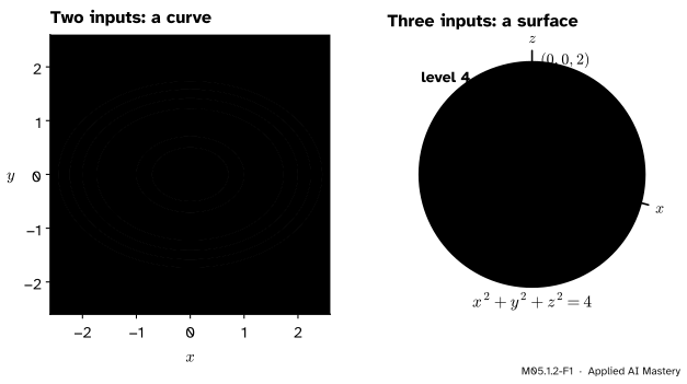
A level set collects the inputs where a function takes one value. With two inputs it is a curve in the plane, here the oval where the running bowl equals 2. With three inputs it is a surface in space, here the sphere where \({x^2 + y^2 + z^2}\) equals 4.
Each extra input adds one dimension to the level set. A function of two inputs has level curves, of three inputs level surfaces, and of \(n\) inputs level sets of \({n - 1}\) dimensions, called hypersurfaces. We cannot draw the last kind, but we can describe it exactly, and for the models of machine learning we often know its shape.
Build it up
Step 1. The bowl: ellipses. For \({f(x, y) = x^2 + 2y^2}\) and \({c > 0}\), M04.10.1 showed that \({x^2 + 2y^2 = c}\) is an ellipse with half-widths \(\sqrt{c}\) along \(x\) and \(\sqrt{c/2}\) along \(y\). At \({c = 2}\) it passes through \({(\pm\sqrt{2}, 0)}\) and \({(0, \pm 1)}\).
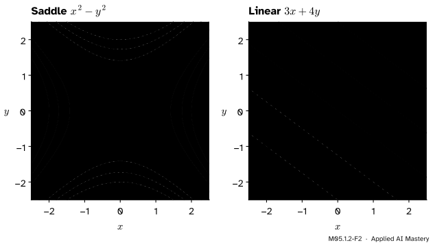
Step 2. The saddle: hyperbolas. For \({h(x, y) = x^2 - y^2}\), the level \({c = 1}\) crosses the \(x\) axis at \({\pm 1}\) and never meets the \(y\) axis, since \({-y^2 = 1}\) has no solution: two curves opening left and right. The level \({c = -1}\) is the same pair turned a quarter turn. The level \({c = 0}\) is \({x^2 = y^2}\), the two lines \({y = x}\) and \({y = -x}\), crossing at the saddle point.
Step 3. A linear function: parallel lines, evenly spaced. For \({g(x, y) = 3x + 4y}\) the level set at \(c\) is the line \({3x + 4y = c}\). Every level has the same slope, so the lines are parallel.
M05.1.2-F2
Left: the saddle’s levels are hyperbolas, except level 0, which is a pair of crossing lines. Right: a linear function’s levels are parallel lines at right angles to its weights, and evenly spaced levels give evenly spaced lines. Negative levels are dashed.
Step 4. Three inputs: spheres. For \({s(x, y, z) = x^2 + y^2 + z^2}\), the square of the distance from the origin, the level \({s = c}\) with \({c > 0}\) is the set of points at distance \(\sqrt{c}\): a sphere of radius \(\sqrt{c}\). In \(\R^n\) the same function \({\norm{\vect{x}}^2}\) has spheres of \({n - 1}\) dimensions as its level sets.
Step 5. Spacing shows steepness, in any dimension. Between the bowl’s levels 1, 2, 3 and 4 the gaps along \(x\) are \({\sqrt{2} - 1 \approx 0.414}\), then 0.318, then 0.268: the levels crowd together as the bowl steepens. The linear function’s gaps never change.
The formal statement
NoteDefinition: level set
Let \({f : D \to \R}\) be a scalar field on a set \(D\) of \(\R^n\), and let \(c\) be a number. The level set of \(f\) at \(c\) is
\[
\{\, \vect{x} \in D : f(\vect{x}) = c \,\} .
\]
For \({n = 2}\) it is also called a level curve or contour line, for \({n = 3}\) a level surface.
Levels never meet. A point in two level sets would have two values, and a function gives each input one. So the level sets of \(f\) split its domain into separate pieces, one for each value in the range.
A level set need not be a curve or a surface. The bowl’s level 0 is the single point \((0, 0)\), and its level \(-1\) is empty. The saddle’s level 0 is two crossing lines. A constant function has one level set, the whole domain. These are the exceptions. For a function whose partial derivatives are continuous, near a point where the gradient of M05.2 is not zero, the level set through it is a smooth curve, surface or hypersurface (the implicit function theorem, stated here without proof), and every exception above sits at a point where the gradient is zero.
A linear function has flat, evenly spaced levels. Take \({g(\vect{x}) = \vect{w}\T\vect{x} + b}\) with \({\vect{w} \neq \vect{0}}\). Two facts follow from the dot product (M02.3).
The levels are at right angles to \(\vect{w}\). If \(\vect{x}_1\) and \(\vect{x}_2\) lie on the same level, then \({\vect{w}\T\vect{x}_1 + b = \vect{w}\T\vect{x}_2 + b}\), so \({\vect{w}\T(\vect{x}_1 - \vect{x}_2) = 0}\): every step within a level is perpendicular to \(\vect{w}\). The level set is a hyperplane: a line in the plane, a plane in space.
The gap between levels \(c\) and \({c + \Delta}\) is \({\Delta / \norm{\vect{w}}}\). Start on level \(c\) and walk a distance \(s\) along the unit vector \({\vect{w} / \norm{\vect{w}}}\), which crosses the levels at right angles. The value changes by
It reaches \({c + \Delta}\) when \({s \norm{\vect{w}} = \Delta}\), that is at \({s = \Delta / \norm{\vect{w}}}\). For \({3x + 4y}\), \({\norm{\vect{w}} = 5}\), so levels 5 apart are one unit apart, as in the figure.
An increasing function keeps the level sets and relabels them. If \(\phi\) is strictly increasing, \({\phi(f(\vect{x})) = \phi(c)}\) exactly when \({f(\vect{x}) = c}\), because a strictly increasing function never takes the same value twice. So \({\phi \circ f}\) has the same level sets as \(f\), with new labels. The spacing of evenly spaced labels can change, though, because \(\phi\) stretches some ranges of values more than others.
Worked example
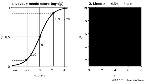
The levels of a logistic model. Lesson ML01.6.4 met the model with score \({z = x_1 + 0.5x_2 - 6}\) and probability \({p = \sigma(z)}\). By the last rule, since \(\sigma\) is strictly increasing, the level sets of \(p\) are the level sets of \(z\): lines.
Which score gives probability \(c\)? Solve \({\sigma(z) = c}\) for \({0 < c < 1}\), one step at a time:
The right-hand side is the logit of \(c\). For \({c = 0.5}\) it is \({\ln 1 = 0}\), for \({c = 0.9}\) it is \({\ln 9 \approx 2.197}\), and for \({c = 0.1}\) it is \({\ln(1/9) \approx -2.197}\).
The lines. The level \({p = c}\) is the line \({x_1 + 0.5x_2 - 6 = \ln\frac{c}{1-c}}\). The decision boundary at threshold 0.5 is \({x_1 + 0.5x_2 = 6}\), through \((3, 6)\), and the level \({p = 0.9}\) is \({x_1 + 0.5x_2 = 8.197}\), through \({(5.197, 6)}\).
The gap. Here \({\norm{\vect{w}} = \sqrt{1 + 0.25} \approx 1.118}\), so the line \({p = 0.9}\) lies \({2.197 / 1.118 \approx 1.965}\) beyond the boundary, on the side \(\vect{w}\) points to.
M05.1.2-F3
The worked example as a trace. Read the sigmoid backwards to turn each probability into a score (left), then draw each score as a line on the map of the features (right).
Evenly spaced probabilities, unevenly spaced lines. The levels \({p = 0.1, 0.3, 0.5, 0.7, 0.9}\) need scores \({-2.197, -0.847, 0, 0.847, 2.197}\). The gaps in score are 1.350, 0.847, 0.847 and 1.350, so the lines crowd round the boundary: the probability changes fastest there, and flattens out far from it.
Code
A level set of a function on a grid: compute the function at every grid point with np.meshgrid, and wherever \({f - c}\) changes sign between two neighbours, the level set crosses the segment between them. A straight line through the two values estimates where.
import numpy as npdef bowl(x, y):return x**2+2* y**2def crossings(f, xs, ys, c):"""Points where f - c changes sign between grid neighbours, placed by linear interpolation.""" X, Y = np.meshgrid(xs, ys) # rows follow ys, columns follow xs G = f(X, Y) - c found = [] a, b = G[:, :-1], G[:, 1:] # neighbours along each row i, j = np.nonzero((a <0) != (b <0)) s = a[i, j] / (a[i, j] - b[i, j]) # how far along the segment the zero lies found.append(np.column_stack([xs[j] + s * (xs[j +1] - xs[j]), ys[i]])) a, b = G[:-1, :], G[1:, :] # neighbours along each column i, j = np.nonzero((a <0) != (b <0)) s = a[i, j] / (a[i, j] - b[i, j]) found.append(np.column_stack([xs[j], ys[i] + s * (ys[i +1] - ys[i])]))return np.vstack(found)for h in (0.25, 0.1, 0.01): xs = np.linspace(-2, 2, round(4/ h) +1) P = crossings(bowl, xs, xs, 2.0) worst = np.abs(bowl(P[:, 0], P[:, 1]) -2).max()print(f"step {h}: {len(P)} points, worst |f - 2| = {worst:.2e}, bound h^2/2 = {h**2/2:.2e}")
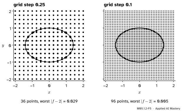
The error shrinks like the square of the step, and never exceeds \({h^2/2}\). The reason: on a straight segment the bowl is a parabola whose second derivative is at most 4 (along \(y\)), and the straight line through two values of such a parabola is off by at most \({4h^2/8}\). A tenth of the step gives a hundredth of the error.
Now the logistic model. Points on the line for \({p = 0.9}\) must all get probability 0.9, and SciPy’s logit is the inverse of expit:
from scipy.special import expit, logitw, b = np.array([1.0, 0.5]), -6.0z9 = logit(0.9)x2 = np.linspace(1, 10, 7)on_line = np.column_stack([6+ z9 -0.5* x2, x2]) # x1 + 0.5 x2 - 6 = logit(0.9)gap = z9 / np.linalg.norm(w)print(round(float(z9), 3), expit(on_line @ w + b).round(6), round(float(gap), 3))print("plugging 0.9 into the score gives p =", round(float(expit(0.9)), 3))
2.197 [0.9 0.9 0.9 0.9 0.9 0.9 0.9] 1.965
plugging 0.9 into the score gives p = 0.711
M05.1.2-F5
The level set at 2, found on two grids. Each vermillion point lies on a segment whose ends fall on opposite sides of the level. Cutting the step from 0.25 to 0.1 cuts the worst error from 0.029 to 0.005, close to the factor \({2.5^2 = 6.25}\) that an error like the square of the step predicts.
Explore
This module’s interactive, the level-set explorer, lives in lesson M05.1.3. Choose the logistic score there and slide the level from 0.1 to 0.9: the highlighted line moves sideways without turning, and it moves fastest per step of the slider far from the boundary.
Pitfalls
M05.1.2-F4
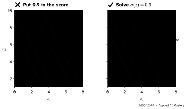
Wrong beside right. Setting the score equal to the probability you want draws a line where the probability is only 0.71. The line for 0.9 is where the score is \({\ln 9 \approx 2.20}\).
“For the line where \(p = 0.9\), set the score to 0.9.”
The score and the probability are different numbers joined by the sigmoid. The level \({p = c}\) is the level \({z = \ln\frac{c}{1 - c}}\) of the score. Even the boundary is not where the score is 0.5: it is where the score is 0.
“A level set is always a curve.”
Usually, not always. The bowl’s level 0 is a single point, its negative levels are empty, the saddle’s level 0 is two lines that cross, and a function that is flat on a region has that whole region as one level set. A contour routine that draws lines will show none of these faithfully.
“The level set is a curve on the surface.”
The level set is a set of inputs, so it lies in the plane of the inputs (or in \(\R^n\)). The curve on the surface at height \(c\) sits directly above it, in \(\R^{n+1}\). Keeping them apart is what lets level sets work for three inputs or a million, where there is no surface to draw.
Check yourself
Recall
1. Define the level set of \(f\) at \(c\). Where does it live?
Show answer
The set of inputs \(\vect{x}\) in the domain with \({f(\vect{x}) = c}\). It lives in the input space \(\R^n\), not on the graph.
2. What are the level sets of \({x^2 + y^2 + z^2}\)?
Show answer
For \({c > 0}\), spheres of radius \(\sqrt{c}\) centred at the origin; for \({c = 0}\) the origin alone; for \({c < 0}\) nothing.
3. What is the saddle’s level set at 0?
Show answer
The two lines \({y = x}\) and \({y = -x}\), since \({x^2 - y^2 = 0}\) means \({x^2 = y^2}\).
4. How far apart are the levels \(c\) and \({c + \Delta}\) of \({\vect{w}\T\vect{x} + b}\)?
Show answer
\({\Delta / \norm{\vect{w}}}\), measured at right angles to the levels, along \(\vect{w}\).
5. Which score \(z\) gives a logistic probability of 0.9, and why is the decision boundary at \({z = 0}\)?
Show answer
\({z = \ln(0.9/0.1) = \ln 9 \approx 2.197}\). The boundary is the level \({p = 0.5}\), and \({\ln(0.5/0.5) = 0}\).
Exercises
1.★ Describe the level sets of \({g(x, y, z) = x + 2y + 2z}\), and find the distance between its levels 0 and 6.
Show solution
They are the parallel planes \({x + 2y + 2z = c}\), at right angles to \({\vect{w} = (1, 2, 2)}\). Here \({\norm{\vect{w}} = \sqrt{1 + 4 + 4} = 3}\), so the levels 0 and 6 are \({6 / 3 = 2}\) apart.
2.★★ Find every level set of \({q(x, y) = e^{-(x^2 + 2y^2)}}\), and the one at \({c = 0.5}\).
Show solution
The values of \(q\) lie in \({0 < q \le 1}\), so for \({c \le 0}\) or \({c > 1}\) the level set is empty. For \({0 < c \le 1}\), take logarithms: \({q = c}\) exactly when \({x^2 + 2y^2 = -\ln c}\). At \({c = 1}\) that is the origin alone. For \({0 < c < 1}\) it is the bowl’s ellipse at height \({-\ln c > 0}\); at \({c = 0.5}\), the ellipse \({x^2 + 2y^2 = \ln 2 \approx 0.693}\). The function \({u \mapsto e^{-u}}\) is decreasing, so \(q\) has the bowl’s level sets in reverse order.
3.★★★ A two-class softmax gives class 1 the probability \({p_1 = e^{z_1}/(e^{z_1} + e^{z_2})}\), with scores \({z_1 = x}\) and \({z_2 = y + 1}\). Show that \({p_1 = \sigma(z_1 - z_2)}\), find the decision boundary \({p_1 = 1/2}\), and find the level \({p_1 = 0.9}\).
Here \({z_1 - z_2 = x - y - 1}\). Since \(\sigma\) is strictly increasing, \({p_1 = 1/2}\) exactly when \({x - y - 1 = 0}\): the line \({y = x - 1}\). The level \({p_1 = 0.9}\) is \({x - y - 1 = \ln 9}\), the parallel line \({y = x - 1 - \ln 9 \approx x - 3.197}\), a distance \({\ln 9 / \sqrt{2} \approx 1.554}\) from the boundary.
Summary card
A level set gathers the inputs where \(f\) takes one value: a curve, a surface, a hypersurface.
M05.1.2-F1
One value, all its inputs.
Level set:\({\{\vect{x} : f(\vect{x}) = c\}}\), a subset of the inputs.
Linear \(f\): hyperplanes at right angles to \(\vect{w}\), gap \({\Delta / \norm{\vect{w}}}\).
Logistic model:\({p = c}\) is \({\vect{w}\T\vect{x} + b = \ln\frac{c}{1 - c}}\); the boundary is score 0.
Spacing: crowded levels mean fast change.
Sources and next steps
Sources. Each was opened and checked against this lesson on 15 November 2026.
Gilbert Strang and Edwin Herman, Calculus Volume 3 (OpenStax), Section 4.1: the level curve of \(f\) at \(c\) is the set of points where \({f(x, y) = c}\), a contour map shows several of them, and a level surface of a function of three variables is the set of points where \({f(x, y, z) = c}\) (with Example 4.7, a hyperboloid).
SciPy reference, scipy.special.expit: the logistic sigmoid \({1/(1 + e^{-x})}\), the inverse of the logit function, applied element-wise.
NumPy 2.5 reference, numpy.meshgrid: with the default Cartesian indexing the outputs have one row for each value of the second input.