Uncertainty for a model’s test-set score without a formula: a bootstrap interval for AUC, the paired bootstrap that compares two models on the same resampled test sets, and permutation_test_score to ask whether a model has learned anything at all.
S02.8.4L2 Intermediate25 minIn review (what this means)
The maths and code on this page are checked by automated tests on every change, but an independent reader has not signed it off yet. Spot a mistake or a confusing step? Tell us.
Compute a bootstrap percentile interval for a test-set AUC by resampling the test examples.
Explain why two models compared on one test set need the paired bootstrap, and derive why its interval for the difference is narrower.
Run sklearn.model_selection.permutation_test_score and read its p-value as a test of whether a model beats chance.
Say which source of variation each method measures, and name bagging and permutation importance as later uses of the same ideas.
The question
On the diabetes table of S01.8, a logistic regression that uses only body mass index predicts which patients’ disease progressed (score above the median, 140.5) with test-set AUC 0.806. One that uses all ten measurements gets 0.842. The test set has 133 patients. Is the bigger model really better, or would another 133 patients have reversed the order? And how sure is the 0.842 itself?
From the last lesson
1. A permutation test with \({K = 9{,}999}\) shuffles finds none as extreme as the data. What p-value do you report?
Show answer
\({(0 + 1)/(9{,}999 + 1) = 0.0001}\), never 0.
2. Six analysts are each timed with two tools. How should a permutation test shuffle?
Show answer
Within each analyst only: swap the two labels of a pair, which flips the sign of that analyst’s difference. That gives \({2^6 = 64}\) relabellings (permutation_type="samples").
Intuition
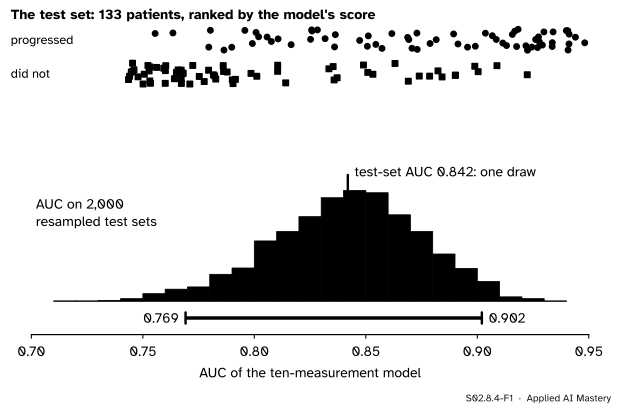
A test set is a sample of the cases the model will meet, so its score is a statistic with a sampling distribution (S02.1.1). The model is fixed once trained; what could have come out differently is which patients landed in the test set. Resample those, rescore, and the spread of the scores is the uncertainty in the 0.842.
S02.8.4-F1
The test-set AUC of the ten-measurement model, 0.842, and its bootstrap distribution over 2,000 resampled test sets. The 95 percent percentile interval runs from 0.769 to 0.902.
The interval is about 0.13 wide. That is the honest size of “AUC 0.84” on 133 patients, and it is why a leaderboard gap of 0.01 on a test set of this size says nothing.
Build it up
Step 1. Freeze the model. Train once and record every test patient’s score. Resampling never refits the model: it asks how the score of this model varies with the test patients.
Step 2. Resample the test rows. Draw 133 row numbers with replacement, take those patients’ labels and scores together, and recompute the AUC. Repeat 2,000 times and read off the percentile interval of S02.8.2.
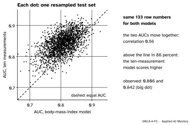
Step 3. Two models: one set of row numbers. To compare the models, use the same resampled rows for both, and record the difference of the two AUCs. This is the paired bootstrap. A resample that happens to hold easy patients flatters both models at once, and the difference cancels that luck out.
S02.8.4-F2
The paired bootstrap. Each dot is one resampled test set scored by both models. The cloud leans along the diagonal: when one model’s AUC is high, so is the other’s.
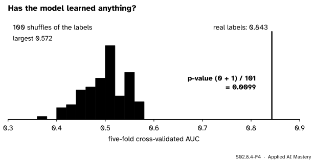
Step 4. A different question: has it learned anything? A permutation test (S02.8.3) shuffles the labels against the features, refits the model on each shuffle, and asks whether the real score beats scores that are pure chance. That tests the null hypothesis of no relation at all, not the size of the score.
The formal statement
The AUC (ML01.7.3) of scores \(s\) on \(n_1\) positives and \(n_0\) negatives is the share of (positive, negative) pairs in the right order:
where \({I(s_i > s_j)}\) is 1 when the positive scores higher, one half for a tie, and 0 when the negative scores higher. It is the Mann-Whitney \(U\) divided by \({n_1 n_0}\) (S02.7.4). In a resample a row drawn twice counts in twice as many pairs.
Why pairing narrows the interval. Write \(\hat{A}_1\) and \(\hat{A}_2\) for the two models’ AUCs on a resampled test set. For any two random variables (M06.10),
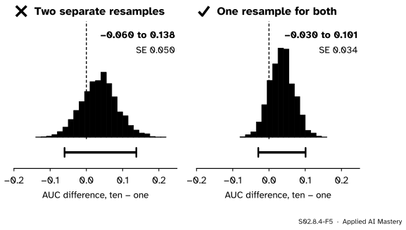
Scored on the same rows, the two AUCs have positive covariance, so the difference varies less than it would if the two were independent. Scored on separately drawn rows, the covariance is 0 and the variances simply add. With the bootstrap standard errors 0.0377 and 0.0334 and correlation 0.56 found below, the three terms are
separate, it is \({\sqrt{0.00142 + 0.00112}} = 0.050\).
Notepermutation_test_score
For a model, data \(\mat{X}\) and labels \(\vect{y}\), compute the cross-validated score \(S_0\). Then for \({k = 1, \dots, K}\) shuffle \(\vect{y}\), refit and score by the same cross-validation, giving \(S_k\). With \(C\) the number of shuffled scores at least \(S_0\),
\[
\text{p-value} = \frac{C + 1}{K + 1},
\]
the \({(b + 1)/(K + 1)}\) rule of S02.8.3. The null hypothesis is that features and labels are independent: the model has nothing to learn.
Go deeper: what these intervals leave out
The bootstrap of the test set holds the trained model fixed. A different training sample would give a different model and a different score, a second source of variation that resampling the test set cannot see. Measuring it means refitting: cross-validation repeated with different splits, or bootstrapping the training set and refitting each time, which is what bagging does on purpose to average that variation away (ML02.2). Statements such as “model 2 beats model 1 on this test set” are about these fitted models; “method 2 beats method 1” needs the refits too.
Worked example
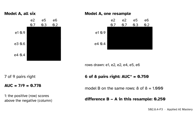
An AUC by hand. Six test examples; e1, e3 and e4 progressed (positives), e2, e5 and e6 did not. Model A scores them 0.9, 0.7, 0.6, 0.4, 0.3 and 0.2 for e1 to e6. There are \({3 \times 3 = 9}\) (positive, negative) pairs. e1 (0.9) beats all three negatives. e3 (0.6) and e4 (0.4) each beat e5 (0.3) and e6 (0.2) but lose to e2 (0.7). So 7 of 9 pairs are right: \({\text{AUC} = 7/9 = 0.778}\).
S02.8.4-F3
The worked example as a trace: the pairs grid on the six examples, then on one resample, where the duplicated e2 appears twice and e3 is missing.
One resample. Suppose the draws are e1, e2, e2, e4, e5, e6. Now the positives are e1 and e4, and the negatives e2 (twice), e5 and e6: \({2 \times 4 = 8}\) pairs. e1 wins all four; e4 loses to both copies of e2 and beats e5 and e6. So \({\text{AUC}^* = 6/8 = 0.750}\).
Pairing. A second model B scores the six 0.8, 0.5, 0.7, 0.6, 0.4 and 0.1. Every positive is above every negative, on the full set and on the resample: AUC 1. On the resample the difference is \({1 - 0.750 = 0.250}\); on the full set it was \({1 - 0.778 = 0.222}\). Repeating this for thousands of resamples, always with one set of rows for both models, gives the paired bootstrap distribution of the difference.
Code
Two models on one test set, as in the question:
import numpy as npfrom scipy import statsfrom sklearn.datasets import load_diabetesfrom sklearn.linear_model import LogisticRegressionfrom sklearn.metrics import roc_auc_scorefrom sklearn.model_selection import StratifiedKFold, permutation_test_score, train_test_splitfrom sklearn.pipeline import make_pipelinefrom sklearn.preprocessing import StandardScalertable = load_diabetes(as_frame=True, scaled=False).frameX = table.drop(columns="target")z = (table["target"] > table["target"].median()).astype(int).to_numpy() # progressed: 1X_tr, X_te, z_tr, z_te = train_test_split(X, z, test_size=0.3, random_state=0, stratify=z)one = make_pipeline(StandardScaler(), LogisticRegression()).fit(X_tr[["bmi"]], z_tr)ten = make_pipeline(StandardScaler(), LogisticRegression()).fit(X_tr, z_tr)s1 = one.predict_proba(X_te[["bmi"]])[:, 1]s2 = ten.predict_proba(X_te)[:, 1]def auc(score, label, axis=-1):"""Share of (positive, negative) pairs in the right order, from ranks (Mann-Whitney U).""" r = stats.rankdata(score, axis=axis) n1 = label.sum(axis=axis) n0 = label.shape[axis] - n1return ((r * label).sum(axis=axis) - n1 * (n1 +1) /2) / (n1 * n0)print(f"{z.sum()} of {len(z)} progressed; test set {len(z_te)} with {z_te.sum()} positives")print(f"AUC: body mass index {auc(s1, z_te):.3f}, ten measurements {auc(s2, z_te):.3f}")
221 of 442 progressed; test set 133 with 66 positives
AUC: body mass index 0.806, ten measurements 0.842
The bootstrap, paired: one array of row numbers serves both models.
K =2000rows = np.random.default_rng(0).integers(0, len(z_te), size=(K, len(z_te)))a1 = auc(s1[rows], z_te[rows], axis=1)a2 = auc(s2[rows], z_te[rows], axis=1)diff = a2 - a1for name, reps in (("body mass index", a1), ("ten measurements", a2), ("difference", diff)): lo, hi = np.percentile(reps, [2.5, 97.5])print(f"{name:>16}: {lo:.3f} to {hi:.3f}, SE {reps.std(ddof=1):.4f}")print(f"correlation of the two AUCs {np.corrcoef(a1, a2)[0, 1]:.2f}; "f"simpler model at least as good in {np.mean(diff <=0):.1%} of resamples")other = np.random.default_rng(1).integers(0, len(z_te), size=(K, len(z_te)))separate = auc(s2[other], z_te[other], axis=1) - a1 # the mistake: separate rows for each modelprint(f"separate resamples: {np.percentile(separate, 2.5):.3f} to {np.percentile(separate, 97.5):.3f}")
 body mass index: 0.728 to 0.877, SE 0.0377
ten measurements: 0.769 to 0.902, SE 0.0334
      difference: -0.030 to 0.101, SE 0.0335
correlation of the two AUCs 0.56; simpler model at least as good in 14.3% of resamples
separate resamples: -0.060 to 0.138
The interval for the gain, \({-0.030}\) to 0.101, contains 0: on 133 patients the data cannot rule out that the two models rank equally well, though the bigger model wins in 86 percent of resamples. Whether the ten-measurement model learned anything at all is a sharper question:
cv = StratifiedKFold(5, shuffle=True, random_state=0)score, null, p = permutation_test_score(make_pipeline(StandardScaler(), LogisticRegression()), X, z, scoring="roc_auc", cv=cv, n_permutations=100, random_state=0)print(f"cross-validated AUC {score:.3f}; shuffled labels: mean {null.mean():.3f}, largest {null.max():.3f}; "f"p-value {p:.4f}")
cross-validated AUC 0.843; shuffled labels: mean 0.499, largest 0.572; p-value 0.0099
S02.8.4-F4
permutation_test_score: with shuffled labels the model scores about 0.5, chance. The real score beats all 100 shuffles, so the p-value is the smallest this run allows, 1/101.
Explore
The module’s resampling machine is in lesson S02.8.1. Its two modes are the two tools of this lesson in miniature: resampling rows to measure how much a statistic varies, and shuffling labels to ask whether a difference is more than chance.
Pitfalls
S02.8.4-F5
Wrong beside right. Resampling the test set separately for each model throws away the pairing and makes the difference look about one and a half times as uncertain as it is.
“The two intervals overlap, so the models are equally good.”
Two separate intervals, 0.728 to 0.877 and 0.769 to 0.902, overlap heavily, yet the question is about the difference, and both models were scored on the same patients. Bootstrap the difference with one set of rows for both. Comparing separate intervals, or resampling each model’s test set on its own, treats the shared patients as if they were different people, the unpaired mistake of S02.7.1.
“A small p-value from permutation_test_score means the model is good.”
It means the model is better than chance, which a model with AUC 0.6 can also be. The size of the score, with its interval, says how good. Ojala and Garriga add that this test cannot tell whether the model uses the relations between features; it only checks for some link between features and labels.
“Bootstrap the test set after tuning on it.”
If the test set chose the model or its threshold, its score is optimistic before any resampling, and the bootstrap faithfully reproduces that optimism. Resampling measures noise, not bias: tune on validation data and keep the test set for the final, single score (ML01.2).
Frontier note: where resampling goes next in machine learning
Bagging (ML02.2) fits one model per bootstrap resample of the training set and averages them, turning the variation this lesson measures into a lower-variance prediction; the rows a resample leaves out, about 37 percent by lesson S02.8.1, give a free “out-of-bag” test set. Permutation importance (ML04.9, R02.3) shuffles one feature column of the test set and measures how much the score drops: a permutation of a single column instead of the labels. Koehn applied the paired bootstrap to test sentences to compare machine-translation systems, and the same recipe serves any metric computed on a shared test set.
Check yourself
Recall
1. When we bootstrap a test-set AUC, what is held fixed and what is resampled?
Show answer
The trained model, and so every test example’s score, is fixed. The test examples are resampled, each with its label and score together.
2. What is the paired bootstrap?
Show answer
Resampling the test rows once per replicate and scoring both models on the same rows, so that the replicate is the difference of their scores on one resampled test set.
3. Why is the paired interval for a difference narrower than one from separate resamples?
Show answer
The variance of the difference is the sum of the two variances minus twice their covariance, and on shared rows the covariance is positive. Separate resamples set it to 0.
4. What null hypothesis does permutation_test_score test, and how is its p-value computed?
Show answer
That features and labels are independent. With \(C\) of \(K\) shuffled-label scores at least the real one, the p-value is \({(C + 1)/(K + 1)}\).
5. What source of variation does a bootstrap of the test set miss?
Show answer
The variation from training: a different training sample would give a different model. Measuring that needs refitting, as in repeated cross-validation or bagging.
Exercises
1.★ A test set has two positives with scores 0.8 and 0.3 and three negatives with scores 0.6, 0.2 and 0.1. Compute the AUC.
Show solution
There are \({2 \times 3 = 6}\) pairs. 0.8 beats all three negatives; 0.3 beats 0.2 and 0.1 but not 0.6. So 5 of 6 pairs are right: AUC \({= 5/6 = 0.833}\).
2.★★ In the exercise above, a resample draws the rows with scores 0.8, 0.8, 0.6, 0.2 and 0.2 (the positive at 0.8 twice, the negative at 0.2 twice). Compute the resample’s AUC.
Show solution
Positives: 0.8 and 0.8. Negatives: 0.6, 0.2 and 0.2. That is \({2 \times 3 = 6}\) pairs, and each copy of 0.8 beats every negative, so all 6 are right: \({\text{AUC}^* = 1}\). The weak positive at 0.3 was left out, and the resample flatters the model.
3.★★★ Two models’ bootstrap AUCs have standard errors 0.030 and 0.040. Find the standard error of their difference if the AUCs are scored on separate resamples, and if they are paired with correlation 0.8. How much narrower is the paired 95 percent interval, roughly?
Fixed model. Test-set resampling ignores training variation.
Sources and next steps
Sources. Each was opened and checked against this lesson on 15 November 2026.
Philipp Koehn, Statistical significance tests for machine translation evaluation, Proceedings of EMNLP 2004, pages 388 to 395. Section 6, Paired Bootstrap Resampling, draws new test sets with replacement, scores both systems on each, and counts how often one beats the other.
Markus Ojala and Gemma C. Garriga, Permutation tests for studying classifier performance, Journal of Machine Learning Research 11 (2010), 1833 to 1863. Definition 1 gives the permutation p-value with one added to numerator and denominator; section 3.1 defines Test 1, which permutes the labels, and Test 2, which permutes features within each class.
scikit-learn, sklearn.model_selection.permutation_test_score: the arguments cv, scoring, n_permutations (default 100) and random_state, the p-value \({(C + 1)/(n_{\text{permutations}} + 1)}\), and that it implements Test 1 of Ojala and Garriga.
Next. Module S02.9, Multiple testing, asks what happens to p-values like these when many models, features or metrics are tested at once. Bagging, the bootstrap applied to the training set, is in ML02.2.