One recipe, write the log-likelihood, differentiate, solve and check, finds the maximum likelihood estimate for Poisson counts and exponential waiting times. The uniform needs a look at the whole curve instead. Then the invariance property, and why an MLE can be biased.
S02.3.2L2 Intermediate25 minIn review (what this means)
The maths and code on this page are checked by automated tests on every change, but an independent reader has not signed it off yet. Spot a mistake or a confusing step? Tell us.
Apply the four-step recipe to derive the maximum likelihood estimates of a Poisson mean and an exponential rate.
Find the MLE of the upper end of a uniform distribution from the shape of the likelihood, where the derivative is never zero.
Use the invariance property to get the MLE of a function of a parameter, such as the mean waiting time 1 / lambda.
Show by simulation that an MLE can be biased, using 1 / x-bar for an exponential rate and the maximum for a uniform.
The question
Five waiting times at a help desk, in minutes, are 1, 3, 0.5, 2.5 and 3 (invented). If waits are exponential with an unknown rate \(\lambda\), which rate makes these five most probable? And what should we do when the same recipe meets a family, like the uniform, where setting a derivative to zero gives no answer at all? Most probabilistic models in machine learning, from a Poisson model of click counts to a classifier, are fitted by asking this question.
From the last lesson
1. What is the MLE of the chance of heads after 7 heads in 10 tosses, and why may we maximise the log-likelihood instead of the likelihood?
Show answer
\({\hat{p} = 7/10 = 0.7}\). The logarithm is increasing, so the likelihood and its logarithm peak at the same value.
2. Is the likelihood \(\mathcal{L}(p)\) the probability that the chance of heads equals \(p\)?
Show answer
No. It is the probability of the observed data given \(p\). Its area is not even 1; it supports comparing two values of \(p\) by a ratio.
Intuition
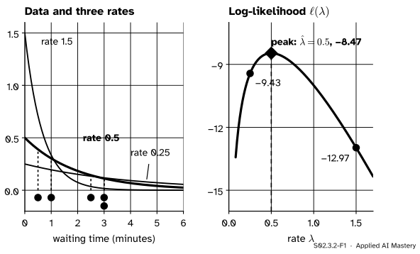
Each candidate rate draws its own density curve over the time axis. The likelihood of a rate is the product of the heights of its curve at the five observed times. A steep curve (a high rate) is tall near zero but almost flat by 3 minutes, where two of the waits sit. A shallow curve (a low rate) reaches the long waits but is low everywhere. The best rate balances the two.
S02.3.2-F1
Left: the five waiting times under three exponential rates. The likelihood multiplies the heights of a curve at the data (dashed for rate 0.5). Right: the log-likelihood of the rate peaks at \({\hat{\lambda} = 0.5}\) per minute, one over the mean wait of 2 minutes.
The log-likelihoods of the three rates are \(-9.43\), \(-8.47\) and \(-12.97\). Rate 0.5 explains the data \({e^{-8.47 + 9.43} \approx 2.6}\) times better than rate 0.25, and about 91 times better than rate 1.5.
Build it up
Lesson S02.3.1 found the coin’s estimate in four moves. They form a recipe that works for every family with a smooth likelihood.
S02.3.2-F2
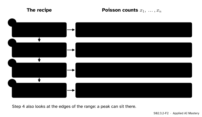
The recipe, run on Poisson counts. Write the log-likelihood as a sum over the data, differentiate, solve for the flat point, and check that it is the top.
Step 1. Write \(\ell\). A Poisson count has probability \({\lambda^x e^{-\lambda} / x!}\). For independent counts \({x_1, \dots, x_n}\) the log-likelihood is the sum of the logs:
Step 3. Solve.\({\ell'(\lambda) = 0}\) gives \({\sum x_i = n\lambda}\), so \({\cmodel{\hat{\lambda}} = \sum \cdata{x_i} / n = \bar{x}}\): the MLE of a Poisson mean is the sample mean.
Step 4. Check.\({\ell''(\lambda) = -\sum x_i / \lambda^2}\) is negative whenever some count is positive, so the curve bends down everywhere and the flat point is the top.
For the errors logged by a service in six one-hour windows (invented), 2, 0, 3, 1, 4, 2, the sum is 12 and \({\hat{\lambda} = 12/6 = 2}\) errors an hour.
The formal statement
NoteThree MLEs and a property
For independent observations \({x_1, \dots, x_n}\):
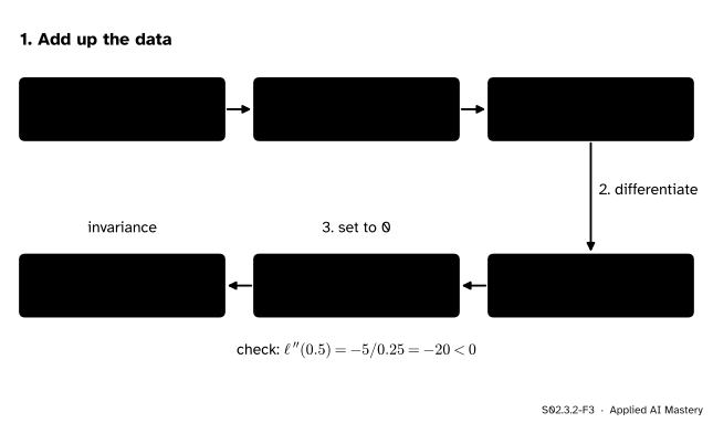
Then \({\ell'(\lambda) = n/\lambda - \sum x_i}\), which is zero when \({\lambda = n / \sum x_i = 1/\bar{x}}\), and \({\ell''(\lambda) = -n/\lambda^2 < 0}\), so this is the top. A density is not a probability, but the recipe uses it in the same way: lesson S02.3.3’s normal works the same.
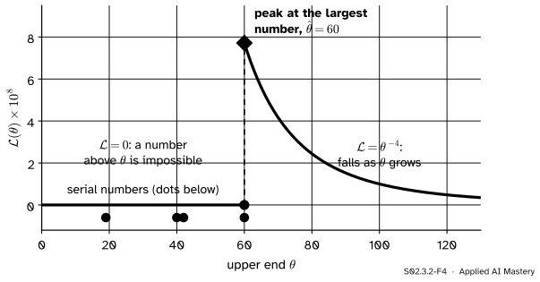
The uniform: a peak on the edge. On \({[0, \theta]}\) the density is \({1/\theta}\) for \({0 \le x \le \theta}\) and 0 outside. If every observation is at most \(\theta\), the likelihood is \({(1/\theta)^n = \theta^{-n}}\). If any observation is above \(\theta\), that observation was impossible, and the likelihood is 0. So
Where it is positive, \(\theta^{-n}\) falls as \(\theta\) grows, so the best value is the smallest \(\theta\) allowed: \({\hat{\theta} = \max_i x_i}\).
S02.3.2-F4
The likelihood of the upper end \(\theta\) for the serial numbers 19, 40, 42, 60. It is zero until \(\theta\) reaches the largest number, jumps, and then falls. The top is at the edge, \({\hat{\theta} = 60}\), where the derivative is not zero.
The serial numbers 19, 40, 42, 60 of the German tank problem (S02.2.4) give \({\hat{\theta} = 60}\). Lesson S02.2.4 showed that the maximum is biased low: it can never exceed \(\theta\), so it usually falls short. For a uniform on \({[0, \theta]}\) its average is \({n\theta / (n + 1)}\), which is \({0.8\,\theta}\) for \({n = 4}\).
Invariance. Write \({\eta = g(\theta)}\) with \(g\) one-to-one. A value of \(\eta\) is the same model as the value \({g^{-1}(\eta)}\) of \(\theta\), so its likelihood is \({\mathcal{L}(g^{-1}(\eta))}\). That is largest when \({g^{-1}(\eta) = \hat{\theta}}\), that is, when \({\eta = g(\hat{\theta})}\). The mean waiting time is \({1/\lambda}\), so its MLE is \({1/\hat{\lambda} = 2}\) minutes, with no new calculus.
MLEs can be biased. For the exponential rate, a sum of \(n\) independent exponential times has a known distribution (a gamma, the family of S02.3.4), and from it
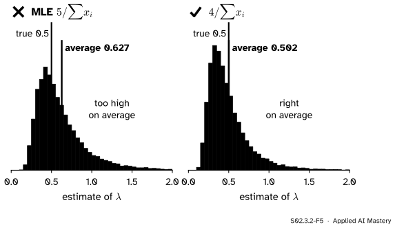
So \({1/\bar{X}}\) is too high on average by a factor \({n/(n - 1)}\): \({5/4 = 1.25}\) for five waiting times. The estimator \({(n - 1) / \sum X_i}\) is unbiased. The bias fades as \(n\) grows, which is typical of maximum likelihood.
Go deeper: the expectation of 1 / x-bar for exponential data
The sum \({S = \sum X_i}\) of \(n\) independent exponential(\(\lambda\)) times has the density \({\lambda^n s^{n-1} e^{-\lambda s} / (n - 1)!}\) for \({s > 0}\), a fact we use here without proof. Call that density \({f_n(s)}\). Dividing it by \(s\) lowers the power of \(s\) by one, and \({(n - 1)! = (n - 1)\,(n - 2)!}\), so
Differentiate and solve.\({\ell'(\lambda) = 5/\lambda - 10 = 0}\) gives \({\hat{\lambda} = 5/10 = 0.5}\) per minute.
Check.\({\ell''(0.5) = -5/0.5^2 = -20 < 0}\), a peak. Its height is \({\ell(0.5) = 5 \ln 0.5 - 5 = -8.47}\).
Invariance. The MLE of the mean wait \({1/\lambda}\) is \({1/0.5 = 2}\) minutes, the sample mean.
Bias. For five times, \({1/\bar{X}}\) averages \({1.25\,\lambda}\), so if the true rate were 0.5 the estimates would average 0.625. The unbiased \({4/\sum x_i}\) gives \({4/10 = 0.4}\) here.
Code
From scratch: the recipe’s answers, checked against a grid search of each log-likelihood.
import numpy as npwait = np.array([1, 3, 0.5, 2.5, 3])counts = np.array([2, 0, 3, 1, 4, 2])tanks = np.array([19, 40, 42, 60])def ell_exp(lam):returnlen(wait) * np.log(lam) - lam * wait.sum()def ell_poisson(lam): # without the sum of ln x!, which has no lambda in itreturn counts.sum() * np.log(lam) -len(counts) * lamgrid = np.linspace(0.001, 6, 6000)lam_hat = grid[np.argmax(ell_exp(grid))]mu_hat = grid[np.argmax(ell_poisson(grid))]theta_hat = tanks.max()print("exponential rate:", round(float(lam_hat), 3), " formula 1/mean:", 1/ wait.mean())print("mean wait by invariance:", 1/ (1/ wait.mean()), " Poisson mean:", round(float(mu_hat), 3))print("ell at 0.25, 0.5, 1.5:", [round(float(ell_exp(r)), 2) for r in (0.25, 0.5, 1.5)])print("uniform upper end:", theta_hat, " likelihood there:", theta_hat **-4.0)
exponential rate: 0.5  formula 1/mean: 0.5
mean wait by invariance: 2.0   Poisson mean: 2.0
ell at 0.25, 0.5, 1.5: [-9.43, -8.47, -12.97]
uniform upper end: 60   likelihood there: 7.71604938271605e-08
Now the bias, by simulation: 20,000 samples of five waiting times with true rate 0.5, and 20,000 samples of four serial numbers from a uniform on \({[0, 100]}\).
rng = np.random.default_rng(5)sums = rng.exponential(1/0.5, size=(20000, 5)).sum(axis=1)print("average of 1/x-bar:", round(float(np.mean(5/ sums)), 3), " theory 0.625")print("average of 4/sum: ", round(float(np.mean(4/ sums)), 3), " theory 0.5")rng = np.random.default_rng(6)maxima = rng.uniform(0, 100, size=(20000, 4)).max(axis=1)print("average maximum:", round(float(maxima.mean()), 1), " theory 4 x 100 / 5 = 80")
average of 1/x-bar: 0.627   theory 0.625
average of 4/sum:   0.502   theory 0.5
average maximum: 80.0   theory 4 x 100 / 5 = 80
The library: scipy.stats.expon.fit and scipy.stats.uniform.fit maximise the likelihood numerically. SciPy writes the exponential with a scale, the mean \({1/\lambda}\), and with a location; fixing the location at 0 with floc=0 gives the model of this lesson.
from scipy import statsloc, scale = stats.expon.fit(wait, floc=0)u_loc, u_scale = stats.uniform.fit(tanks, floc=0)print("expon.fit scale:", round(scale, 6), " so the rate is", round(1/ scale, 6))print("uniform.fit upper end:", round(u_loc + u_scale, 6))
expon.fit scale: 2.0  so the rate is 0.5
uniform.fit upper end: 60.0
SciPy reports the scale 2, the mean wait, which is the invariance property at work: maximising over the scale or over the rate picks out the same model.
Explore
This module’s interactive, the likelihood surface explorer, is in lesson S02.3.3. One thing to try by hand first: add a sixth waiting time of 10 minutes. The sum becomes 20 and \(n\) becomes 6, so the rate estimate drops to \({6/20 = 0.3}\) and the mean wait rises to 3.33 minutes. One long wait moves the estimate a lot, because the MLE here depends on the data only through their mean.
Pitfalls
S02.3.2-F5
Wrong beside right, in a seeded simulation. The MLE \({1/\bar{x}}\) of an exponential rate from five times averages about 0.627 (0.625 in theory) when the truth is 0.5. Using \({n - 1}\) in place of \(n\) removes the bias.
“The maximum likelihood estimate is unbiased.”
Often it is not. \({1/\bar{x}}\) overshoots an exponential rate by the factor \({n/(n - 1)}\), the sample maximum undershoots the end of a uniform by \({n/(n + 1)}\), and lesson S02.3.3 finds that the normal MLE of \(\sigma^2\) divides by \(n\). Maximum likelihood is chosen for other strengths: it works for any model you can write down, it homes in on the truth as the sample grows, and in smooth models (not the uniform, whose range moves with \(\theta\)) its variance comes down to the smallest that any unbiased estimator can have (S02.10).
“Set the derivative to zero and solve: that is always the answer.”
Only when the peak is a smooth flat point inside the allowed range. The uniform’s likelihood \({\theta^{-n}}\) has derivative \({-n\theta^{-n-1}}\), never zero; solving would find nothing, or tempt you to send \(\theta\) off to infinity. Draw the likelihood, including the places where it is zero, and look for the top. The coin with 0 heads (S02.3.1, exercise 2) has its peak on an edge too.
“Invariance means unbiasedness carries over.”
Invariance is about where the peak is, not about averages. \({\bar{x}}\) is an unbiased estimate of the mean wait, yet \({1/\bar{x}}\) is a biased estimate of the rate: the average of \(1/\bar{X}\) is not one over the average of \(\bar{X}\).
Check yourself
Recall
1. What are the four steps of the recipe for an MLE?
Show answer
Write the log-likelihood as a sum over the data, differentiate, solve for the flat point, and check that it is the top (second derivative negative), looking at the edges of the range too.
2. What is the MLE of a Poisson mean, and of an exponential rate?
Show answer
\({\hat{\lambda} = \bar{x}}\) for the Poisson and \({\hat{\lambda} = 1/\bar{x}}\) for the exponential.
3. Why does the derivative not find the MLE of the upper end of a uniform?
Show answer
Where the likelihood is positive it is \({\theta^{-n}}\), which falls steadily, so its derivative is never zero. The top is at the edge of the allowed values, \({\hat{\theta} = \max x_i}\).
4. The rate estimate of the waiting times is 0.5 per minute. What is the MLE of the mean wait, and which property gives it?
Show answer
\({1/0.5 = 2}\) minutes, by invariance: the MLE of \({g(\theta)}\) is \({g(\hat{\theta})}\).
5. For five exponential times, what does \({1/\bar{X}}\) average, as a multiple of the true rate?
Show answer
\({5/4 = 1.25}\) times the true rate; in general \({n/(n - 1)}\) times.
Exercises
1.★ A web page gets 3, 5, 2, 6 and 4 sign-ups on five days (invented). Assuming Poisson counts, find the MLE of the daily mean and the MLE of the chance of a day with no sign-ups, \({e^{-\lambda}}\).
Show solution
\({\hat{\lambda} = (3 + 5 + 2 + 6 + 4)/5 = 4}\). By invariance the MLE of \({e^{-\lambda}}\) is \({e^{-4} \approx 0.0183}\).
2.★★ A Bernoulli variable is 1 with chance \(p\) and 0 otherwise. For observations \({x_1, \dots, x_n}\) of 0s and 1s, derive the MLE of \(p\) with the recipe, and say what it means for a classifier’s test-set accuracy.
Show solution
Each observation has probability \({p^{x_i}(1 - p)^{1 - x_i}}\), so
This is the coin’s log-likelihood with \({k = \sum x_i}\), so \({\hat{p} = \sum x_i / n = \bar{x}}\), with \({\ell'' < 0}\) as in S02.3.1. Scoring each test example 1 if the classifier is right and 0 if not, the MLE of its accuracy is the share it got right, such as 0.9 for 90 of 100.
3.★★★ Data \({x_1, \dots, x_n}\) come from the density \({\theta x^{\theta - 1}}\) on \({[0, 1]}\), with \({\theta > 0}\). Derive the MLE of \(\theta\), and evaluate it for the data 0.5, 0.8, 0.9.
which is positive because every \({\ln x_i < 0}\). The check: \({\ell''(\theta) = -n/\theta^2 < 0}\). For the data, \(\sum \ln x_i = \ln 0.5 + \ln 0.8 + \ln 0.9 = -1.0217\), so \(\hat{\theta} = 3/1.0217 \approx 2.94\).
Summary card
Write \(\ell\), differentiate, solve, check, and look at the edges.
S02.3.2-F1
The waiting times choose rate 0.5.
Poisson.\({\hat{\lambda} = \bar{x}}\). Exponential.\({\hat{\lambda} = 1/\bar{x}}\); 0.5 for the waiting times.
Uniform on \({[0, \theta]}\).\({\hat{\theta} = \max x_i}\): a peak on the edge.
Invariance. The MLE of \({g(\theta)}\) is \({g(\hat{\theta})}\): mean wait \({1/0.5 = 2}\).
Bias.\({\E[1/\bar{X}] = n\lambda/(n - 1)}\); MLEs can be biased.
Sources and next steps
Sources. Each was opened and checked against this lesson on 15 November 2026.
Jeremy Orloff and Jonathan Bloom, Reading 10b: Maximum Likelihood Estimates, MIT OpenCourseWare 18.05, Spring 2022. Example 3 (light bulbs) finds the exponential MLE as the reciprocal of the sample mean; Example 5 finds the MLE of a uniform’s ends without calculus, as the smallest and largest observations; the Appendix states the invariance property.
Philippe Rigollet, Maximum Likelihood Estimation, MIT OpenCourseWare 18.650, Fall 2016, slides. The examples slide lists the Bernoulli and Poisson MLEs as the sample mean.
SciPy documentation, rv_continuous.fit: maximum likelihood is the default method, and floc holds the location parameter fixed.